Interviews are more than just a Q&A session—they’re a chance to prove your worth. This blog dives into essential Robust Control interview questions and expert tips to help you align your answers with what hiring managers are looking for. Start preparing to shine!
Questions Asked in Robust Control Interview
Q 1. Explain the concept of robust stability and performance.
Robust stability and performance in control systems mean the ability of a system to maintain stability and desired performance levels even in the presence of uncertainties. Think of it like building a bridge – you design it to withstand expected loads (wind, traffic), but robust design ensures it remains stable and functional even with unexpected events (earthquakes, heavier-than-expected vehicles). In control systems, these uncertainties can stem from inaccurate model parameters, external disturbances, or component variations.
Robust stability guarantees that the closed-loop system remains stable despite these uncertainties. Robust performance goes a step further, ensuring the system meets specified performance requirements (e.g., settling time, overshoot) under the same uncertain conditions. Achieving both is crucial for reliable system operation in real-world applications.
Q 2. What are the limitations of classical control methods in handling uncertainties?
Classical control methods, like PID controllers, excel in designing controllers for systems with well-defined, accurate models. However, they struggle significantly when facing uncertainties. They often rely on linearized models around operating points, ignoring nonlinearities and variations. A slight deviation from the assumed model can lead to instability or poor performance. For instance, a PID controller tuned for a specific plant model might perform poorly if the plant parameters change due to temperature variations or aging. They lack systematic ways to account for uncertainty bounds and guarantee stability and performance under those conditions.
Q 3. Describe the different types of uncertainties encountered in control systems.
Uncertainties in control systems can be broadly classified into several types:
- Parameter uncertainties: These involve variations in the system’s physical parameters (e.g., mass, inertia, resistance) due to manufacturing tolerances, aging, or environmental factors. For example, the resistance of a resistor in an electrical circuit might deviate from its nominal value.
- Unmodeled dynamics: Real systems are often more complex than their mathematical models. Unmodeled dynamics represent the neglected parts of the system, which can significantly impact performance. For instance, a simplified model of a robot arm may ignore friction forces.
- External disturbances: These are unpredictable inputs that affect the system’s behavior (e.g., wind gusts on an aircraft, load variations in a power system). These can push the system away from its desired operating point.
- Sensor noise: Measurements from sensors are rarely perfect and often contain noise. This noise can corrupt feedback signals, impacting controller performance.
- Actuator limitations: Actuators (motors, valves, etc.) have limitations like saturation and rate limits. These constraints can affect the control system’s ability to achieve the desired behavior.
Understanding the types and sources of uncertainty is crucial for designing a robust controller.
Q 4. Explain the concept of H-infinity control and its advantages.
H-infinity (H∞) control is a powerful robust control technique that minimizes the worst-case effect of uncertainties on the system’s performance. It focuses on finding a controller that guarantees stability and performance within a specified range of uncertainty. Imagine a shield protecting a system from the worst possible attack (uncertainty). The ‘infinity’ in H∞ refers to the worst-case scenario considered in the optimization process.
Advantages of H∞ control:
- Guaranteed robustness: It explicitly considers uncertainties and guarantees stability and performance within predefined bounds.
- Handles multiple uncertainties: It can address various types of uncertainties simultaneously (parameter variations, disturbances, etc.).
- Systematic design procedure: It provides a structured framework for controller design based on mathematical optimization techniques.
H∞ control is widely used in applications requiring high reliability and performance in uncertain environments.
Q 5. How do you design an H-infinity controller for a given system?
Designing an H∞ controller involves several steps:
- System modeling: Create a state-space model of the plant, including uncertainties represented through weighting functions. These weighting functions shape the frequency response of the uncertainties.
- Weighting function selection: Carefully choose weighting functions to capture the frequency characteristics of the uncertainties and specify desired performance levels (e.g., disturbance rejection, tracking accuracy).
- H∞ optimization: Use H∞ synthesis techniques (e.g., Riccati equations, Linear Matrix Inequalities (LMIs)) to find the controller that minimizes the H∞ norm of the closed-loop transfer function relating disturbances and uncertainties to performance outputs.
- Controller implementation: Implement the resulting controller in the physical system.
- Validation: Validate the controller’s performance through simulations and experiments, considering various scenarios with uncertainties.
Specialized software tools (e.g., MATLAB’s Robust Control Toolbox) are frequently used to perform the optimization and implementation steps.
Q 6. Explain the concept of Linear Quadratic Regulator (LQR) control.
The Linear Quadratic Regulator (LQR) is an optimal control technique that minimizes a quadratic cost function while considering state and control input penalties. Imagine you want to drive a car to a parking spot smoothly. LQR allows you to define the cost of deviation from the spot (state penalty) and the cost of sharp turns or acceleration (control input penalty). The controller finds the optimal path that minimizes the overall cost.
The LQR controller calculates the optimal control input based on the current state of the system and the cost function parameters (weighting matrices Q and R). Matrix Q weighs the state deviations, while matrix R weighs the control effort. The solution involves solving a Riccati equation.
Q 7. How do you tune an LQR controller?
Tuning an LQR controller involves adjusting the weighting matrices Q and R in the cost function. These matrices determine the relative importance given to state regulation and control effort. There’s no single ‘best’ tuning method, but a common approach is:
- Start with a reasonable initial guess: Begin with diagonal matrices Q and R, where the diagonal elements reflect the relative importance of each state and control input. For example, if precise tracking of a particular state is crucial, you might assign a larger weight to that state in Q.
- Iterative adjustment: Systematically adjust the elements of Q and R, observing the system’s response. Increasing elements in Q emphasizes reducing state error, possibly leading to higher control effort. Increasing elements in R prioritizes minimizing control effort, potentially sacrificing some tracking accuracy.
- Simulation and testing: Extensive simulation is crucial for evaluating the controller’s performance and determining the optimal balance between state regulation and control effort.
- Consider performance indices: Monitor metrics like settling time, overshoot, and control effort to assess the controller’s performance. This feedback guides the tuning process.
Trial and error, along with experience and understanding of the system dynamics, are essential for effective LQR tuning. Systematic methods like pole placement and eigenvalue analysis can also assist in tuning.
Q 8. What are the advantages and disadvantages of LQR control?
Linear Quadratic Regulator (LQR) is a powerful optimal control technique for linear systems. It minimizes a quadratic cost function, balancing control effort and state deviation from a desired trajectory.
- Advantages: LQR is computationally efficient, guaranteeing stability if the system is controllable and the cost function is positive definite. It provides a systematic way to tune controller performance by adjusting weighting matrices in the cost function. For example, increasing the weight on state error improves tracking, while increasing the weight on control effort reduces actuator usage.
- Disadvantages: LQR is limited to linear systems. It doesn’t inherently handle constraints on states or control inputs, which is a significant limitation in real-world applications. It also assumes perfect knowledge of the system dynamics, which is rarely the case. For example, an LQR controller designed for a robot arm might not perform well if the arm’s inertia changes due to carrying a heavier load.
Q 9. Explain the concept of Model Predictive Control (MPC).
Model Predictive Control (MPC) is an advanced control strategy that uses a model of the system to predict its future behavior over a finite time horizon (the prediction horizon). At each time step, MPC solves an optimization problem to find the optimal control sequence that minimizes a cost function over the prediction horizon, subject to constraints. Only the first control input in this optimal sequence is implemented, and then the process is repeated at the next time step using updated measurements. Think of it like a chess player who plans several moves ahead, but only makes the first move before reconsidering the situation based on the opponent’s response.
Imagine you are driving a car. MPC uses a model of your car’s dynamics (how it accelerates, brakes, steers) to predict how your actions (steering angle, throttle, brake pressure) will affect its trajectory over the next few seconds. It then calculates the best combination of actions to reach your destination while adhering to speed limits and avoiding obstacles.
Q 10. How does MPC handle constraints?
MPC’s strength lies in its ability to explicitly handle constraints. These constraints, which might include limits on actuator inputs (e.g., maximum torque of a motor), state variables (e.g., maximum speed of a vehicle), or output variables (e.g., maximum temperature of a reactor), are directly incorporated into the optimization problem. The optimization solver then finds the best control sequence that satisfies all these constraints while minimizing the cost function. This is typically done using quadratic programming (QP) or other numerical optimization techniques. For instance, in a chemical process, MPC can ensure that pressure and temperature remain within safe operating ranges even during disturbances.
Q 11. What are the advantages and disadvantages of MPC?
- Advantages: MPC can handle multivariable systems and constraints effectively. It’s also adaptable to changing operating conditions and disturbances. Its ability to anticipate future behavior makes it suitable for systems with significant delays or non-minimum phase characteristics.
- Disadvantages: MPC can be computationally intensive, particularly for systems with many states and constraints. The accuracy of the predictions and control performance depends heavily on the accuracy of the system model. Poor model accuracy leads to suboptimal or unstable control. MPC also requires careful tuning of the prediction horizon, control horizon, and weighting matrices in the cost function. An improperly tuned MPC controller can be unstable or perform poorly.
Q 12. Compare and contrast LQR and MPC.
Both LQR and MPC are powerful control techniques, but they differ significantly in their approach:
- LQR is an optimal control method for linear systems without constraints, yielding a simple, feedback control law. It’s computationally efficient but lacks the ability to handle constraints.
- MPC is an optimal control method that can handle constraints and non-linear systems (through linearization or other approximations). It’s computationally more demanding but offers superior performance in the presence of constraints and disturbances.
In essence, LQR provides an elegant solution for simple linear systems, while MPC is a more versatile and powerful tool for complex systems with constraints, though at the cost of increased computational complexity. The choice depends on the specific application and its requirements.
Q 13. Explain the role of uncertainty modeling in robust control design.
Uncertainty modeling is crucial in robust control design because real-world systems are never perfectly known. Model inaccuracies, external disturbances, and parameter variations can significantly affect a controller’s performance, leading to instability or poor tracking. Robust control aims to design controllers that are insensitive to these uncertainties. This involves incorporating uncertainty into the control design process, so the controller can effectively manage these deviations. For example, a robust autopilot for an aircraft must account for variations in wind speed and aircraft mass to maintain stable flight.
Q 14. Describe different methods for uncertainty modeling (e.g., parametric, non-parametric).
Several methods exist for uncertainty modeling:
- Parametric Uncertainty: This approach models uncertainty as variations in system parameters. For example, the mass of a robot arm might be known to lie within a certain range. The controller is then designed to work effectively within this parameter range. This is often represented using intervals or probability distributions.
- Non-parametric Uncertainty: This method doesn’t explicitly model parameter variations but instead considers the uncertainty as additive or multiplicative noise affecting the system’s dynamics or outputs. This approach is useful when the exact nature of the uncertainty is unknown or difficult to quantify. Techniques like H-infinity control are particularly adept at dealing with this type of uncertainty.
- Set-membership Uncertainty: This approach describes the uncertainty as belonging to a known set. This is often used when there are bounds on the uncertainties, for instance, when sensors might have a known level of inaccuracy.
The choice of uncertainty modeling method depends on the available knowledge about the system and the level of conservatism desired. More detailed uncertainty models generally lead to more robust controllers but can also increase computational complexity.
Q 15. How do you handle time-varying uncertainties?
Handling time-varying uncertainties in robust control is a significant challenge because the system’s dynamics change over time, making it difficult to design a controller that guarantees stability and performance across all possible variations. Imagine trying to balance a ball on your fingertip – if your finger’s position changes unpredictably, maintaining balance becomes much harder. Similarly, in a control system, unexpected changes in parameters like mass, friction, or external disturbances can destabilize the system.
Several approaches exist to address this:
Adaptive Control: This approach uses online estimation of the time-varying parameters to adjust the controller’s gains continuously. Think of it as constantly recalibrating your finger’s position to maintain balance as the ball shifts.
Gain Scheduling: This method involves designing multiple controllers for different operating points or parameter ranges. The controller is then switched or interpolated between these designs based on the current system state. This is like having multiple strategies for balancing the ball – one for slow movements, another for fast ones.
Robust Control with Time-Varying Uncertainty Models: This approach involves explicitly modeling the time-varying uncertainties within a robust control framework (e.g., using Linear Parameter-Varying (LPV) models or time-varying Linear Matrix Inequalities (LMIs)). The controller is designed to guarantee stability and performance in spite of the variations described by the model. This is the most mathematically rigorous method, providing guarantees of performance under certain assumptions about the rate of variation.
The choice of method depends on the specific application, the nature of the uncertainties, and the available computational resources.
Career Expert Tips:
- Ace those interviews! Prepare effectively by reviewing the Top 50 Most Common Interview Questions on ResumeGemini.
- Navigate your job search with confidence! Explore a wide range of Career Tips on ResumeGemini. Learn about common challenges and recommendations to overcome them.
- Craft the perfect resume! Master the Art of Resume Writing with ResumeGemini’s guide. Showcase your unique qualifications and achievements effectively.
- Don’t miss out on holiday savings! Build your dream resume with ResumeGemini’s ATS optimized templates.
Q 16. What are the different types of robust stability analysis techniques?
Robust stability analysis techniques aim to assess a system’s stability in the presence of uncertainties. Different techniques cater to various types of uncertainties and complexities.
Small Gain Theorem: This classic theorem is used to analyze systems with unstructured uncertainties, represented as multiplicative or additive perturbations. It provides conditions for stability based on the gain of the uncertainty and the complementary sensitivity function of the nominal closed-loop system.
H∞ Control: This approach seeks to minimize the worst-case effect of uncertainties on the system’s performance, often by minimizing a specific H∞ norm. It is particularly useful for dealing with frequency-dependent uncertainties.
μ-Analysis and Synthesis: This sophisticated technique accounts for structured uncertainties, allowing for more accurate modeling of real-world scenarios. It uses a structured singular value (μ) to measure the robustness of the system.
Linear Matrix Inequalities (LMIs): LMIs provide a powerful tool for formulating and solving robust stability and performance problems. Many robust control problems can be expressed as LMI feasibility or optimization problems, enabling efficient numerical solutions.
Lyapunov-based Methods: These methods involve finding a Lyapunov function that satisfies certain conditions to guarantee stability, even in the presence of uncertainties. We’ll delve deeper into this in a later answer.
The choice of technique depends heavily on the nature and structure of the uncertainties in the system model.
Q 17. Explain the concept of robust performance.
Robust performance goes beyond just ensuring stability in the face of uncertainties; it requires that the system continues to meet its performance specifications even when uncertainties are present. Think of a self-driving car – it must not only stay on the road (stability) but also maintain a safe following distance and reach its destination efficiently (performance), regardless of variations in road conditions, traffic, or sensor accuracy.
Robust performance is typically quantified by ensuring that certain performance measures remain within acceptable bounds despite the uncertainties. This might involve specifications on the system’s frequency response, transient response, or other relevant performance metrics.
In mathematical terms, this can be achieved using methods like H∞ control, which ensures that the closed-loop transfer function satisfies certain bounds across the frequency range, even under the influence of uncertainties.
Q 18. How do you verify robust stability and performance?
Verification of robust stability and performance involves several methods, often used in combination.
Simulation: Running Monte Carlo simulations with various uncertainty realizations allows us to observe the system’s behavior under a wide range of conditions. This provides an empirical assessment of robustness.
Frequency-domain analysis: Techniques like Bode plots and Nyquist plots can be used to visualize the system’s sensitivity to uncertainties and evaluate robustness margins (gain and phase margins discussed later).
Numerical methods: Using software tools that solve LMIs or perform μ-analysis provides a more rigorous mathematical verification of robust stability and performance. These often leverage the underlying mathematical conditions associated with specific theorems.
Experimental testing: Real-world testing on a physical prototype, or a high-fidelity simulation representing the real world, can help validate theoretical analysis and confirm robustness under actual operating conditions. This is particularly important before deployment.
The specific methods chosen will depend on the system complexity, the nature of uncertainties, and the required level of confidence in the robustness results.
Q 19. Describe the use of Lyapunov functions in robust control.
Lyapunov functions are a cornerstone of stability analysis in robust control. They provide a powerful mathematical tool to prove the stability of a system, even in the presence of uncertainties. Imagine a ball rolling downhill – its potential energy decreases as it rolls down. A Lyapunov function is analogous to potential energy; if it decreases along the system’s trajectories, the system is guaranteed to be stable.
In the context of robust control, Lyapunov functions are used to establish stability conditions that hold for a range of parameter variations. By finding a Lyapunov function that satisfies certain inequalities (often expressed as LMIs), we can guarantee stability for the entire uncertainty set.
For example, finding a positive definite Lyapunov function V(x) such that its derivative along the system trajectories, dV/dt, is negative definite for all uncertainties within a specified set, proves the robust stability of the system. This is mathematically expressed using inequalities involving the system matrices and the Lyapunov function.
Q 20. What are the different types of robustness margins (e.g., gain margin, phase margin)?
Robustness margins quantify the amount of uncertainty a system can tolerate before losing stability. These margins provide a useful measure of the system’s robustness.
Gain Margin: This represents the factor by which the system’s open-loop gain can be increased or decreased before instability occurs. A large gain margin indicates robustness to gain variations.
Phase Margin: This indicates the amount of additional phase lag that can be introduced into the open-loop transfer function before instability occurs. A large phase margin suggests resilience to phase shifts introduced by uncertainties or delays.
Other robustness margins exist, often defined based on the specific types of uncertainties being considered. For instance, in H∞ control, the H∞ norm of the closed-loop transfer function acts as a robustness margin.
Q 21. How do you determine robustness margins for a given control system?
Determining robustness margins typically involves frequency-domain analysis. For gain and phase margins:
Obtain the open-loop transfer function: This is the transfer function of the system without the feedback controller.
Plot the Bode plot: This plot shows the magnitude and phase of the open-loop transfer function as a function of frequency.
Find the gain crossover frequency (ωgc): This is the frequency at which the magnitude of the open-loop transfer function is 1 (0 dB).
Determine the phase margin (PM): This is the difference between the phase at ωgc and -180 degrees. A larger PM indicates greater robustness.
Determine the gain margin (GM): This is the amount by which the open-loop gain can be increased or decreased at ωgc before the phase reaches -180 degrees. A larger GM indicates greater robustness.
For more complex systems with structured uncertainties, numerical techniques like μ-analysis are used to determine the robustness margins, which are often represented as a structured singular value.
Software tools such as MATLAB provide functions to easily calculate these margins from a given system model. It’s important to remember that margins are only indicators of robustness and don’t guarantee stability under all circumstances; particularly when the assumptions made in their derivation are violated.
Q 22. Explain the concept of loop shaping in robust control design.
Loop shaping in robust control design is a powerful technique used to adjust the frequency response of a control system to achieve desired performance and robustness characteristics. Think of it like tuning a musical instrument – you’re adjusting the system’s response at different frequencies to get the ‘sound’ you want. Instead of focusing on specific parameters, loop shaping directly manipulates the open-loop transfer function to meet performance requirements such as minimizing steady-state error, maximizing bandwidth, and ensuring sufficient phase margin for stability. This is typically done graphically using Bode plots or Nyquist plots.
For example, we might want to increase the system’s gain at low frequencies to reduce steady-state error. However, we need to be careful not to introduce excessive gain at high frequencies, which could lead to instability. We strategically shape the open-loop response using compensators (e.g., lead, lag, lead-lag compensators) to achieve the desired balance between performance and robustness. The compensator modifies the open-loop transfer function, impacting the closed-loop response, effectively ‘shaping’ the loop’s behavior. The goal is to create an open-loop transfer function that provides sufficient gain and phase margins across the frequency range of interest, guaranteeing stability and performance even with uncertainty in the plant model.
Q 23. What are the limitations of robust control techniques?
While robust control offers significant advantages, it’s not without limitations. One key limitation is the computational complexity, especially when dealing with high-order systems or complex uncertainty descriptions. Finding optimal controllers can be computationally intensive, potentially requiring significant computing power and time. Furthermore, robust control methods often rely on accurate models of uncertainty. Overly conservative assumptions about uncertainty can lead to overly cautious designs, sacrificing performance. Conversely, underestimating uncertainty can jeopardize the robustness of the system, making it vulnerable to unexpected disturbances.
Another significant limitation lies in handling highly nonlinear systems. Many robust control techniques are based on linear models, and their effectiveness diminishes significantly when faced with strong nonlinearities. Finally, the practical implementation of robust controllers can be challenging. The complexity of the controller can lead to higher hardware costs and increased implementation challenges, especially in embedded systems with limited computational resources.
Q 24. How do you handle nonlinearities in robust control design?
Handling nonlinearities in robust control design presents a significant challenge because many robust control techniques assume linear system models. Several strategies can be employed to address this. One approach is to linearize the nonlinear system around operating points. This creates a linear approximation valid only within a limited operating range. Multiple linear models can then be used to cover a wider operating range, leading to a gain-scheduled controller which adapts its parameters based on the current operating point. Another approach involves using nonlinear robust control techniques such as sliding mode control or adaptive control. These methods explicitly account for system nonlinearities, but often come with increased complexity.
For instance, in a robotic manipulator control application, the dynamics are inherently nonlinear. We might employ a gain-scheduled controller, where different linear controllers are designed for different joint angles and speeds. The controller switches between these linear controllers based on the current state of the robot. Alternatively, a sliding mode controller could be designed to robustly control the robot’s movements despite uncertainties and nonlinearities in the system dynamics. The choice of method depends heavily on the specific nonlinearity, the complexity of the system, and the desired level of performance and robustness.
Q 25. Describe your experience with robust control software tools (e.g., MATLAB, Simulink).
I have extensive experience using MATLAB and Simulink for robust control design and analysis. MATLAB provides powerful tools for modeling, simulating, and analyzing control systems, including functions for designing various robust controllers like H∞ controllers and μ-synthesis controllers. Simulink, its graphical counterpart, allows for the creation of block diagrams that visually represent the control system and facilitates simulations that incorporate real-world complexities like sensor noise and actuator saturation. I’m proficient in using the Robust Control Toolbox within MATLAB, which provides specialized functions for uncertainty modeling, robust controller synthesis, and performance analysis using various robustness metrics like gain and phase margins, singular values, and structured singular values (μ). I frequently leverage these tools for both designing and validating robust controllers in various projects.
For example, I’ve extensively used Simulink’s capabilities to create detailed models of physical systems, incorporating nonlinearities and uncertainties. I’ve used the LMI toolbox in MATLAB to solve optimization problems related to robust control design, such as finding controllers that minimize the H∞ norm of the closed-loop transfer function. My expertise spans from developing simple controllers to implementing more sophisticated techniques for complex systems with multiple uncertainties.
Q 26. Describe a project where you applied robust control techniques. What were the challenges and how did you overcome them?
In a recent project involving the control of a wind turbine, I used robust control techniques to improve the efficiency and stability of energy generation. The challenge was to design a controller that could maintain optimal power capture in the presence of significant wind gust disturbances and uncertainties in the turbine’s aerodynamic parameters. These parameters are affected by factors like wind speed, blade angle, and temperature variations.
To address this challenge, I employed H∞ control design methodology. This method allows for explicitly considering the uncertainties in the model through a structured singular value (μ) analysis. The H∞ controller was designed to minimize the effect of wind gusts on the turbine’s speed and power output while ensuring robust stability. I used simulations in Simulink to verify the controller’s performance under various scenarios, including sudden wind gusts and changes in wind speed and direction. This rigorous simulation process identified limitations and allowed for fine tuning of the controller’s parameters before real-world deployment. The resulting control system showed significantly improved performance in terms of energy capture efficiency and reduced oscillations, leading to a more reliable and efficient wind turbine operation.
Q 27. How do you ensure the robustness of a control system in a real-world application?
Ensuring the robustness of a control system in a real-world application requires a multifaceted approach. Firstly, a thorough understanding of the system and its uncertainties is crucial. This includes identifying potential sources of uncertainty, such as parameter variations, sensor noise, and external disturbances. Secondly, a robust control design methodology should be selected that effectively addresses these uncertainties. This could involve techniques like H∞ control, μ-synthesis, or LQR control with robust weighting functions. Thirdly, rigorous testing and validation are essential to confirm the controller’s performance and robustness under various operating conditions. This includes both simulations under realistic conditions and real-world experiments.
Furthermore, incorporating features such as fault detection and isolation mechanisms and adaptive control strategies enhance robustness. Fault detection allows for early identification of potential problems, enabling timely corrective actions. Adaptive control continuously adjusts controller parameters in response to changing system dynamics and uncertainties, thus maintaining performance over time. Regular monitoring of the system’s performance and health in real-world operation, along with appropriate safety protocols, are also necessary to guarantee the long-term stability and robustness of the control system.
Q 28. Explain the trade-off between performance and robustness in control system design.
The trade-off between performance and robustness in control system design is a fundamental aspect of control engineering. High-performance controllers often strive for fast response times, minimal overshoot, and precise tracking. However, these aggressive designs can be sensitive to uncertainties and disturbances, potentially leading to instability or poor performance in real-world scenarios. Conversely, robust controllers prioritize stability and resilience against uncertainties but might exhibit slower response times or larger steady-state errors. Finding the right balance involves carefully considering the specific application requirements and the characteristics of the uncertainties.
Think of it like driving a car: a highly responsive car provides excellent performance, but aggressive driving in uncertain conditions (e.g., icy roads) can be dangerous. A more stable, less responsive car might offer a safer experience, but might not be as exhilarating. Similarly, in control design, we must find a balance that optimizes both the system’s performance and its ability to withstand unexpected situations. Tools like Bode plots and Nyquist plots are used to visualize and analyze this tradeoff, allowing us to make informed decisions about the controller parameters to achieve a satisfactory compromise between performance and robustness. This often involves using optimization techniques to achieve a controller that strikes the desired balance within a given set of constraints.
Key Topics to Learn for Robust Control Interview
- System Modeling and Representation: Understanding state-space representations, transfer functions, and their limitations in describing real-world systems. Consider exploring different modeling techniques for various applications.
- Stability Analysis: Mastering concepts like Nyquist stability criterion, Bode plots, and root locus methods to determine system stability and robustness. Practical application includes analyzing the stability margins of a control system in the presence of uncertainty.
- Frequency Response Techniques: Gain and phase margins, sensitivity and complementary sensitivity functions, their interpretations and implications for design choices. Think about how these relate to robustness against disturbances and uncertainties.
- Robust Control Design Techniques: Familiarize yourself with H-infinity control, μ-synthesis, and Linear Quadratic Gaussian (LQG) control. Explore practical examples of designing controllers that maintain performance despite parameter variations.
- Uncertainty Modeling: Understanding different types of uncertainties (parametric, unstructured) and how to incorporate them into your control design process. Think about how real-world systems deviate from ideal models.
- Nonlinear Control (Optional): A basic understanding of nonlinear control concepts can be advantageous, especially for advanced roles. This could include feedback linearization or sliding mode control.
- Practical Problem Solving: Develop your ability to formulate control problems, select appropriate design techniques, and critically evaluate the performance of your design using simulations and analysis.
Next Steps
Mastering robust control opens doors to exciting and challenging career opportunities in various industries, from aerospace and automotive to robotics and process control. A strong foundation in this area significantly enhances your value as an engineer. To maximize your job prospects, it’s crucial to present your skills effectively. Creating an ATS-friendly resume is paramount for getting your application noticed. We highly recommend using ResumeGemini to build a professional and impactful resume tailored to your specific experience. Examples of resumes tailored to Robust Control are available within ResumeGemini to help guide your process.
Explore more articles
Users Rating of Our Blogs
Share Your Experience
We value your feedback! Please rate our content and share your thoughts (optional).
What Readers Say About Our Blog
Very informative content, great job.
good
