The right preparation can turn an interview into an opportunity to showcase your expertise. This guide to Advanced Numerical Modeling and Simulation interview questions is your ultimate resource, providing key insights and tips to help you ace your responses and stand out as a top candidate.
Questions Asked in Advanced Numerical Modeling and Simulation Interview
Q 1. Explain the difference between explicit and implicit numerical methods.
Explicit and implicit methods are two fundamental approaches in numerical time integration, crucial for solving time-dependent problems. Imagine you’re trying to predict the position of a ball thrown in the air. An explicit method calculates the next position based solely on the current position and velocity. Think of it like taking a snapshot of the ball’s state and using that to predict the next snapshot. This is simple and computationally inexpensive for each step. However, it has limitations; it needs very small time steps (think high frame rate for a smooth animation) to remain stable and accurate, particularly when dealing with stiff systems. Otherwise, the calculations might diverge from reality—the simulated ball might fly off into space!
An implicit method, in contrast, considers the ball’s position and velocity at both the current and the future time. It solves a system of equations to find the future state. This is like trying to guess the ball’s future state by considering how gravity and other factors will affect it. Implicit methods generally allow for larger time steps but require solving a system of equations at each step, making them computationally more expensive per step. They are often preferred for stiff systems, which are highly sensitive to initial conditions or rapid changes. For example, simulating fluid flow with abrupt changes in velocity would benefit from the stability of an implicit approach.
In short: Explicit methods are simple, fast per step, but require small time steps for stability. Implicit methods are more complex, slower per step, but allow larger time steps and better stability.
Q 2. Describe the Finite Element Method (FEM) and its applications.
The Finite Element Method (FEM) is a powerful numerical technique used to solve partial differential equations (PDEs) that govern many physical phenomena. Imagine dividing a complex shape, like a car chassis, into many small, simple shapes (elements). FEM works by approximating the solution within each element using simple functions (interpolation functions). Then, it connects these solutions across element boundaries to obtain an approximate solution for the entire domain. Think of it like building a complex structure with Lego bricks: each brick is an element, and the way they connect represents the approximation of the solution across boundaries.
FEM finds wide application in various fields. In structural mechanics, it’s used to analyze stress and strain in bridges, buildings, and aircraft components. In fluid dynamics, it simulates the flow of air around an airplane wing or blood flow in arteries. Heat transfer analysis, electromagnetism, and biomechanics are further examples where FEM provides crucial insights.
The versatility of FEM comes from its ability to handle complex geometries and material properties. For instance, FEM enables engineers to simulate the impact of a car crash with high fidelity by considering the different materials and their behavior under stress.
Q 3. What are the advantages and disadvantages of Finite Difference Method (FDM)?
The Finite Difference Method (FDM) is another widely used numerical technique for solving PDEs. It approximates the derivatives in the PDE using difference quotients— essentially, replacing derivatives with differences in function values at nearby points on a grid. Imagine a checkerboard; each square represents a grid point where we approximate the solution.
Advantages: FDM is relatively simple to implement and understand, particularly for problems with regular geometries and simple boundary conditions. It’s computationally efficient for many applications, especially those with simpler geometries.
Disadvantages: FDM struggles with irregular geometries, leading to challenges in representing complex shapes accurately. Accuracy can also be compromised near boundaries. Additionally, it can be difficult to adapt FDM to handle complex material properties or boundary conditions smoothly. For example, applying FDM to a problem involving a fractured material would require a clever and potentially complex way of handling the discontinuity.
Q 4. Explain the concept of mesh refinement in numerical simulations.
Mesh refinement in numerical simulations involves increasing the density of elements or grid points within a specific area of the computational domain. Imagine zooming in on a map: we increase the level of detail in the area of interest. This is crucial for improving accuracy in regions of high gradients or significant changes in the solution. For instance, in simulating fluid flow around an airfoil, we would refine the mesh near the airfoil’s surface where the flow gradients are steepest. Failure to do this can lead to inaccurate results or even instability in the solution.
There are several approaches to mesh refinement: h-refinement involves reducing the element size, p-refinement increases the order of the interpolation functions (improving the accuracy of the approximation within each element), and r-refinement adjusts the location of the grid points. The choice depends on the nature of the problem and the desired balance between accuracy and computational cost.
Q 5. How do you handle boundary conditions in numerical modeling?
Boundary conditions specify the values or behavior of the solution at the boundaries of the computational domain. They are essential for obtaining a physically meaningful solution. Imagine a heat transfer problem: we need to specify the temperature at the boundaries of the object to simulate its thermal behavior correctly. Incorrect or missing boundary conditions will lead to an inaccurate and unphysical solution.
Common types of boundary conditions include: Dirichlet (specifying the value of the solution at the boundary), Neumann (specifying the derivative of the solution at the boundary— for example, the heat flux), and Robin (a combination of Dirichlet and Neumann).
Implementing boundary conditions often involves modifying the system of equations generated by the numerical method. This can involve adding extra equations or modifying existing ones to enforce the specified boundary conditions. For example, in a finite element analysis, this would entail modifying the stiffness matrix and the load vector.
Q 6. What is convergence in numerical simulations, and how do you achieve it?
Convergence in numerical simulations means that as we refine the discretization (e.g., decrease the mesh size or increase the time steps), the numerical solution approaches the true solution of the PDE. It signifies that our method is working correctly and producing accurate results. Think of it as hitting a target: as we refine our approximation, we get closer to the bullseye.
Achieving convergence often involves a combination of techniques. Firstly, you need a stable and consistent numerical method. Secondly, careful selection of the discretization parameters (mesh size, time step) is crucial. Thirdly, using adaptive refinement techniques, as described earlier, focuses computational resources on areas where high accuracy is needed. Finally, convergence checks, such as comparing solutions obtained with different mesh sizes, help determine if the solution has converged to a satisfactory level of accuracy. If the differences between successively refined solutions fall below a certain tolerance, we can consider the simulation converged.
Q 7. Describe different types of numerical errors (truncation, round-off).
Numerical errors are unavoidable in any numerical simulation. They are broadly classified into two categories: truncation error and round-off error.
Truncation error arises from the approximation inherent in numerical methods. We replace continuous functions and derivatives with discrete approximations. Imagine approximating a curve with a series of straight line segments; the deviation from the true curve is truncation error. This error depends on the chosen numerical method and the discretization parameters. Higher-order methods generally have smaller truncation errors.
Round-off error results from the limited precision of computer arithmetic. Computers store numbers with finite precision, introducing small errors in each calculation. These small errors can accumulate over numerous computations, leading to potentially significant errors in the final result, particularly in lengthy simulations. Double-precision arithmetic is often used to mitigate this problem.
Q 8. What are the stability criteria for numerical methods?
Stability criteria in numerical methods ensure that errors don’t amplify during the computation, leading to a meaningful solution. Imagine a snowball rolling downhill – a stable method is like a small snowball that grows at a manageable rate, while an unstable method is like an avalanche, where a tiny initial error explodes into a completely inaccurate result. These criteria often involve constraints on the time step (Δt) and spatial step (Δx) sizes. For example, in explicit time-stepping schemes for solving partial differential equations (PDEs), the Courant-Friedrichs-Lewy (CFL) condition is a crucial stability criterion. The CFL condition states that the numerical domain of dependence must encompass the physical domain of dependence. This essentially means the numerical solution must incorporate information from all relevant areas influenced by the physical process. Violating the CFL condition can lead to oscillations and divergence of the solution. Different numerical methods have different stability criteria, and often, these criteria are derived through von Neumann stability analysis, which involves examining the amplification factor of error modes.
For instance, solving the heat equation using an explicit finite difference scheme requires adhering to a CFL-like condition such as Δt ≤ Δx²/2α where α is the thermal diffusivity. Implicit methods, on the other hand, are often unconditionally stable (meaning they don’t have such strict constraints on Δt and Δx), but they require solving a system of equations at each time step, which can be computationally more expensive.
Q 9. Explain the concept of order of accuracy in numerical methods.
The order of accuracy refers to how well a numerical method approximates the exact solution. Think of it as the precision of a measurement. A higher-order method provides a more accurate solution with less error. It’s expressed using the Big O notation. For example, a method with first-order accuracy (O(Δx)) means the error decreases linearly with the step size. A second-order method (O(Δx²)) means the error decreases quadratically with the step size. This implies that halving the step size in a first-order method halves the error, while halving the step size in a second-order method reduces the error by a factor of four. Consequently, higher-order methods generally require less computational effort to achieve the same level of accuracy.
Consider approximating the derivative of a function f(x) at a point. A first-order forward difference approximation is given by: (f(x+Δx) - f(x))/Δx. This is O(Δx) accurate. A second-order central difference approximation, (f(x+Δx) - f(x-Δx))/(2Δx), is O(Δx²) accurate, offering a significantly improved approximation for the same step size.
Q 10. How do you validate and verify your numerical models?
Validation and verification are crucial steps to ensure the reliability of numerical models. Verification confirms that the computer code correctly implements the numerical method, while validation ensures that the model accurately represents the real-world phenomenon. Verification often involves code testing, unit tests, and comparisons against analytical solutions or known benchmarks with simple geometries. Validation involves comparing the model’s predictions against experimental data or observational data from the real-world system. This comparison is used to quantify the accuracy and reliability of the model under different conditions and inputs.
For example, when modeling fluid flow over an airfoil, verification might involve testing the solver’s ability to conserve mass and momentum in a simple case like Couette flow, where an analytical solution exists. Validation would involve comparing the model’s predictions of lift and drag coefficients with experimental measurements obtained from wind tunnel tests on a similar airfoil. Discrepancies between the model and experimental data can highlight limitations in the model or the experimental setup, guiding model refinements and/or further investigations.
Q 11. What are some common challenges in numerical modeling and how do you address them?
Numerical modeling presents several challenges. Mesh generation for complex geometries can be time-consuming and require significant expertise. Balancing accuracy and computational cost is an ongoing challenge; finer meshes improve accuracy but greatly increase computational demands. Dealing with singularities or discontinuities in the solution (e.g., shocks in fluid flow) necessitates specialized numerical techniques, such as adaptive mesh refinement. Furthermore, accurately modeling multi-physics phenomena, where different physical processes interact (e.g., fluid-structure interaction), requires advanced coupled solvers and careful consideration of coupling algorithms.
Addressing these challenges often involves employing advanced meshing techniques (e.g., unstructured meshes, adaptive mesh refinement), using efficient numerical solvers (e.g., multigrid methods), and incorporating robust error control mechanisms. Choosing the appropriate numerical method (e.g., finite element, finite volume, finite difference) depends on the specific problem and desired level of accuracy. Careful model calibration and validation using experimental data are also essential for reliable simulations.
Q 12. Describe your experience with different software packages for numerical simulation (e.g., ANSYS, Abaqus, COMSOL).
I have extensive experience using ANSYS Fluent, Abaqus, and COMSOL Multiphysics for various numerical simulations. ANSYS Fluent is my go-to tool for CFD simulations, particularly for turbulent flows, where I have leveraged various turbulence models (k-ε, k-ω SST, LES). Abaqus has been instrumental in conducting finite element analysis (FEA) of structural mechanics problems, including linear and nonlinear static and dynamic analyses. My projects involved simulating stress and strain distributions under various loading conditions. COMSOL Multiphysics, with its multi-physics capabilities, has allowed me to model coupled problems such as fluid-structure interaction, heat transfer, and electromagnetics, often in complex geometries requiring careful mesh generation and solver setup. Each package has its strengths and weaknesses. The choice of software depends heavily on the specifics of the problem at hand.
For instance, in a project involving simulating the flow of blood through a human artery, I used ANSYS Fluent to model the fluid flow and COMSOL Multiphysics to couple the fluid dynamics with the structural mechanics of the artery wall, simulating the pulsatile nature of blood flow and its impact on the vessel.
Q 13. Explain your understanding of computational fluid dynamics (CFD).
Computational Fluid Dynamics (CFD) is a branch of fluid mechanics that uses numerical methods and algorithms to solve and analyze problems that involve fluid flows. It involves solving the Navier-Stokes equations, which describe the motion of viscous fluids, along with relevant equations for mass, momentum, and energy conservation. These equations are typically complex, nonlinear partial differential equations that cannot be solved analytically except for simplified cases. CFD employs various discretization techniques, such as finite volume, finite element, or finite difference methods, to approximate the solution on a computational mesh. The solution process involves meshing the computational domain, solving the governing equations numerically, and post-processing the results to visualize and quantify the flow field.
CFD has widespread applications in various fields, including aerospace engineering (designing aircraft wings), automotive engineering (optimizing car aerodynamics), weather forecasting (predicting atmospheric flows), and biomedical engineering (modeling blood flow in arteries). The accuracy and reliability of CFD simulations heavily depend on the chosen numerical methods, turbulence models, and mesh quality. Careful validation with experimental data is crucial for ensuring the fidelity of the simulation.
Q 14. Describe your experience with different turbulence models.
Turbulence modeling is crucial in CFD simulations, as directly resolving all turbulent scales is often computationally prohibitive. I have experience with various turbulence models, including Reynolds-Averaged Navier-Stokes (RANS) models (e.g., k-ε, k-ω SST) and Large Eddy Simulation (LES). RANS models solve time-averaged equations, using turbulence models to close the equations. The k-ε model is a widely used RANS model, but it can struggle in regions with strong streamline curvature or adverse pressure gradients. The k-ω SST model often performs better in such regions and near walls. LES resolves larger turbulent scales directly, while modeling smaller scales using subgrid-scale models. This approach offers higher accuracy than RANS but at significantly higher computational cost. The choice of the turbulence model depends on the specific flow characteristics, computational resources, and desired accuracy. In some cases, hybrid approaches combining RANS and LES (Detached Eddy Simulation or DES) are used.
In a project involving the design of a wind turbine, I compared the performance of k-ε and k-ω SST RANS models. While both provided reasonable predictions of the overall thrust and torque, the k-ω SST model offered better accuracy in predicting the flow separation near the blade tips, which is critical for understanding the turbine’s efficiency. For more detailed flow analysis close to the turbine blade I utilized Detached Eddy Simulation (DES).
Q 15. Explain your understanding of finite volume methods.
Finite Volume Method (FVM) is a discretization technique used in numerical simulations to solve partial differential equations (PDEs). Unlike Finite Difference Methods (FDM) which approximate derivatives at points, FVM integrates the PDE over control volumes, resulting in a balance equation for each volume. Imagine dividing your problem domain (like a fluid flow region) into small cells – these are the control volumes. The FVM then applies conservation laws (e.g., conservation of mass, momentum, energy) to each cell, ensuring that whatever enters a cell must either leave or be stored within it.
This approach is particularly powerful for conservation problems because it inherently preserves the integral form of the conservation law. For example, in fluid dynamics, it ensures that mass is conserved globally, even if there are numerical errors within individual cells. The method involves calculating fluxes (the flow of quantities) across the cell boundaries. Different schemes exist for approximating these fluxes, each with its own strengths and weaknesses regarding accuracy and stability (e.g., upwind, central, and higher-order schemes).
In practice, I’ve used FVM extensively to model turbulent flows in complex geometries, where its inherent conservation properties were crucial for obtaining accurate and physically meaningful results. For instance, in a simulation of airflow around an aircraft wing, FVM accurately captured the lift and drag forces, factors that are directly linked to conservation of momentum.
Career Expert Tips:
- Ace those interviews! Prepare effectively by reviewing the Top 50 Most Common Interview Questions on ResumeGemini.
- Navigate your job search with confidence! Explore a wide range of Career Tips on ResumeGemini. Learn about common challenges and recommendations to overcome them.
- Craft the perfect resume! Master the Art of Resume Writing with ResumeGemini’s guide. Showcase your unique qualifications and achievements effectively.
- Don’t miss out on holiday savings! Build your dream resume with ResumeGemini’s ATS optimized templates.
Q 16. What is the role of mesh independence in numerical simulations?
Mesh independence refers to the state where the solution of a numerical simulation becomes insensitive to further refinement of the computational mesh. Think of the mesh as a grid overlaying your problem domain. A finer mesh means smaller cells, leading to a more accurate representation of the geometry and solution. However, finer meshes come at the cost of increased computational time and resources.
The goal is to achieve a mesh that’s fine enough to capture all relevant details of the solution but not so fine as to be unnecessarily expensive. We determine mesh independence by performing simulations with progressively finer meshes and comparing the results. If the solution converges to a stable value as the mesh is refined, we’ve achieved mesh independence. It’s a crucial step in validating the accuracy and reliability of the simulation results, ensuring that the solution is not an artifact of the chosen mesh resolution but rather a true representation of the underlying physics.
I’ve encountered scenarios where neglecting mesh independence studies led to erroneous conclusions. In one project involving heat transfer in a microfluidic device, initial simulations with a coarse mesh yielded significantly different results compared to those obtained with a finer, mesh-independent solution. This highlighted the importance of thoroughly investigating mesh independence before drawing any meaningful conclusions.
Q 17. How do you choose an appropriate numerical method for a given problem?
Choosing the right numerical method is a critical decision, depending on several factors including the type of PDE, the problem’s geometry, the desired accuracy, and available computational resources. There’s no one-size-fits-all answer. It often involves a careful assessment of the problem’s characteristics.
- Type of PDE: Hyperbolic PDEs (e.g., wave equations) often benefit from methods designed to handle wave propagation accurately, while elliptic PDEs (e.g., Laplace’s equation) may be better suited to iterative solvers. Parabolic PDEs (e.g., heat equation) require methods capable of handling time-dependent behavior.
- Geometry: Complex geometries often necessitate methods like FVM which can handle unstructured meshes more efficiently than FDM. Simple geometries might allow the use of simpler methods such as FDM on structured grids.
- Accuracy Requirements: High-accuracy simulations require higher-order methods, which usually come at a computational cost. Less demanding applications might suffice with lower-order methods.
- Computational Resources: The choice must also consider available computing power. Resource-intensive high-order methods might not be feasible for large-scale problems.
Often, a combination of methods or a hybrid approach proves to be the most effective solution. For example, I might couple a FVM for the fluid flow with a Finite Element Method (FEM) for the structural analysis in a fluid-structure interaction problem.
Q 18. Explain your experience with parallel computing and High-Performance Computing (HPC).
My experience with parallel computing and HPC is extensive. I’ve worked on numerous projects requiring the use of distributed computing architectures to solve computationally demanding simulations. I’m proficient in using MPI (Message Passing Interface) and OpenMP for parallelizing codes, enabling efficient utilization of multi-core processors and clusters of computers.
In one project involving large-eddy simulation (LES) of turbulent flow in a wind turbine, parallelization was crucial. The computational cost of LES is notoriously high, and without parallelization, the simulation would have been impractical. I employed MPI to distribute the computational load across multiple nodes in a high-performance computing cluster, resulting in a significant reduction in simulation time. Moreover, I’ve utilized various HPC tools and libraries for optimizing code performance, such as performance profiling tools to identify bottlenecks and improve scalability.
Understanding load balancing, communication overhead, and data management in parallel environments is critical for achieving optimal performance. I’ve had to address challenges related to data transfer and synchronization between different processors, ensuring efficient communication without compromising accuracy.
Q 19. How do you handle complex geometries in numerical simulations?
Handling complex geometries is a major challenge in numerical simulations. Structured grids, suitable for simple geometries, often fail to adequately represent complex shapes. This is where unstructured meshes come in. Methods such as FVM are well-suited for unstructured meshes, which can conform to intricate shapes by using various element types (triangles, tetrahedra, etc.).
However, unstructured meshes can lead to issues with mesh quality (e.g., distorted elements) which can negatively affect solution accuracy. Careful mesh generation is essential, using appropriate meshing tools and techniques to ensure good mesh quality. Adaptive mesh refinement (AMR) is a valuable technique where the mesh is refined only in regions requiring higher resolution, improving accuracy while controlling computational costs.
Furthermore, boundary condition implementation becomes more challenging with complex geometries. Accurate representation of boundary conditions is vital, often requiring careful consideration of the geometry’s intricacies. I frequently employ boundary-fitted meshes to better capture boundary details and improve the accuracy of boundary condition applications. For instance, in simulating blood flow in the human heart, I would utilize body-fitted unstructured meshes to accurately represent the intricate geometry of the heart chambers and valves.
Q 20. Explain your experience with post-processing and visualization of simulation results.
Post-processing and visualization of simulation results are essential for interpreting the data and extracting meaningful insights. It involves analyzing the raw data generated by the simulation and presenting it in a clear and understandable manner. I’m proficient in using various software packages such as ParaView, Tecplot, and MATLAB for visualizing simulation results.
My workflow typically involves extracting relevant data from the simulation output files, performing necessary calculations (e.g., averaging, filtering, etc.), and creating visualizations such as contour plots, streamlines, and animations. Creating effective visualizations is crucial for communicating complex results to both technical and non-technical audiences. For example, I’ve used animations to demonstrate the evolution of a turbulent flow over time, making complex dynamics easy to understand.
Beyond basic visualizations, I also perform quantitative analysis of the results to extract key performance indicators (KPIs). This might involve calculating average velocities, pressure drops, or forces based on the simulated data. In one project involving heat exchanger design, I used post-processing techniques to optimize the exchanger’s geometry to maximize heat transfer efficiency.
Q 21. Describe your understanding of multiphysics simulations.
Multiphysics simulations involve coupling different physical phenomena within a single simulation. It addresses situations where multiple physical processes interact and influence each other. For example, fluid-structure interaction (FSI), where the flow of a fluid affects the deformation of a structure and vice-versa, is a typical multiphysics problem.
These simulations often require specialized techniques to handle the coupling between different physical domains. Common approaches include staggered and monolithic coupling schemes. Staggered schemes solve each physics separately, iteratively exchanging information between them. Monolithic schemes solve all the physics simultaneously, often resulting in better accuracy but increased computational cost. The choice between these methods depends on the specific problem, the desired accuracy, and the available computational resources.
I’ve experienced working on multiphysics problems, particularly in the area of FSI. For instance, simulating the interaction between blood flow and arterial walls necessitated a coupled model, accurately representing the pulsatile blood flow and the resulting wall deformation. These models often require advanced numerical techniques and specialized software to handle the complex interactions between different physical domains, and meticulous validation is critical to ensure accuracy.
Q 22. How do you ensure the accuracy and reliability of your simulation results?
Ensuring accuracy and reliability in simulation results is paramount. It’s a multifaceted process that begins even before the simulation starts. We need to meticulously validate our model against experimental data or established theoretical frameworks. This involves comparing the simulation outputs with known results under various conditions, identifying discrepancies and refining the model accordingly. Think of it like testing a recipe – you wouldn’t serve a dish without tasting it first!
Beyond model validation, crucial aspects include:
- Mesh Refinement/Grid Convergence Studies: For finite element or finite difference methods, reducing the element size (mesh refinement) improves accuracy but increases computational cost. A grid convergence study systematically refines the mesh until the solution converges to a stable value, indicating sufficient accuracy.
- Numerical Method Selection: Different numerical methods have different strengths and weaknesses regarding accuracy and stability. Choosing the appropriate method (e.g., implicit vs. explicit time integration) for the specific problem is crucial. An inappropriate choice could lead to inaccurate or unstable solutions.
- Error Estimation and Control: Estimating and controlling various sources of errors (truncation, round-off, discretization) is vital. Techniques like Richardson extrapolation can estimate the error and guide mesh refinement.
- Verification and Validation: Verification ensures the code is implementing the model correctly. Validation checks if the model accurately reflects the real-world system.
For example, in a fluid dynamics simulation, I would perform a grid convergence study to ensure the results are independent of the mesh size. I would also validate the simulation against experimental data from wind tunnel tests, adjusting model parameters as needed to achieve good agreement.
Q 23. Explain your approach to solving a non-linear problem using numerical methods.
Solving non-linear problems numerically often requires iterative methods because a direct solution is usually impossible. The core idea is to start with an initial guess for the solution and iteratively refine it until a convergence criterion is met. Think of it like finding the top of a hill by taking small steps uphill—eventually, you’ll reach the summit (the solution).
Common approaches include:
- Newton-Raphson Method: This method uses the derivative of the non-linear equation to find the root iteratively. It’s fast when close to the solution but can be sensitive to the initial guess.
- Fixed-Point Iteration: This method rearranges the equation into a fixed-point form and iteratively applies the function until convergence. It’s simpler than Newton-Raphson but can converge more slowly.
- Picard Iteration: This method is particularly useful for solving non-linear systems of equations. It involves iteratively solving a linearized version of the system.
The choice of method depends on the specific problem’s characteristics. For instance, in simulating a heat transfer problem with temperature-dependent material properties (a non-linearity), I might employ a Newton-Raphson approach because of its generally faster convergence. Convergence criteria are usually based on the change in the solution between iterations or the residual of the equations, where the iteration stops when the change or residual is below a predefined tolerance.
Q 24. Describe your experience with optimization techniques in numerical simulations.
Optimization techniques are indispensable in numerical simulations, particularly when dealing with inverse problems or parameter estimation. They help find the optimal values of model parameters that best fit experimental data or minimize a certain objective function. Imagine trying to tune a musical instrument – you adjust different parameters (strings, tuning pegs) until it produces the desired sound.
I have experience with several optimization algorithms, including:
- Gradient-based methods (e.g., steepest descent, conjugate gradient): These methods use the gradient of the objective function to iteratively move towards the optimum. They are efficient when the objective function is smooth and differentiable.
- Derivative-free methods (e.g., Nelder-Mead, genetic algorithms): These methods don’t require gradient information, making them suitable for non-smooth or noisy objective functions. Genetic algorithms, in particular, are robust but can be computationally expensive.
- Simulated annealing: This method uses a probabilistic approach to escape local optima and find the global optimum. It’s effective for complex, highly non-linear problems.
For example, in a groundwater flow model, I’ve used optimization to estimate hydraulic conductivity parameters by minimizing the difference between simulated and observed water levels. The choice of optimization algorithm depends on the complexity of the objective function and the computational resources available.
Q 25. Explain your experience with uncertainty quantification in numerical simulations.
Uncertainty quantification (UQ) is crucial for understanding the reliability of simulation results because input parameters, model structure, and numerical methods themselves all introduce uncertainties. Instead of a single deterministic output, UQ provides a probability distribution of potential outcomes, giving a much more complete picture.
My experience encompasses several UQ methods, including:
- Monte Carlo simulation: This involves generating multiple random samples of input parameters and running the simulation for each sample. The resulting outputs form a statistical distribution of the results, quantifying the uncertainty.
- Stochastic Finite Element Method (SFEM): This method directly incorporates uncertainty into the mathematical model using stochastic variables. It’s particularly useful when the uncertainty in input parameters is represented by probability distributions.
- Polynomial Chaos Expansion (PCE): This technique approximates the response of the system as a polynomial function of random variables, providing efficient uncertainty propagation.
In a structural mechanics simulation, for example, I would use Monte Carlo simulation to assess the impact of uncertain material properties on the predicted stress levels, providing a range of potential failure probabilities rather than a single point estimate.
Q 26. How do you handle discontinuities in numerical models?
Discontinuities in numerical models present significant challenges, as standard numerical methods often struggle to handle sharp changes accurately. Techniques employed to address these challenges depend heavily on the type of discontinuity and the governing equations.
Strategies for handling discontinuities include:
- Mesh refinement: Concentrating mesh elements around the discontinuity can significantly improve accuracy. This allows the numerical solution to better capture the sharp change.
- Adaptive mesh refinement (AMR): This technique automatically refines the mesh in regions where the solution exhibits high gradients or discontinuities. It’s computationally efficient, as refinement is only applied where needed.
- Special numerical methods: Methods such as the immersed boundary method or the level set method are specifically designed to handle discontinuities effectively. These methods often involve tracking the location of the discontinuity and applying special numerical treatments near it.
- Shock-capturing schemes: For problems involving shocks (strong discontinuities), specialized numerical schemes such as Godunov’s method or essentially non-oscillatory (ENO) schemes are used to avoid oscillations and ensure stability.
For instance, in simulating crack propagation in a solid, I would use adaptive mesh refinement to focus the mesh around the crack tip, improving the accuracy of the stress field calculations and facilitating the simulation of crack growth.
Q 27. Describe your experience with model calibration and parameter estimation.
Model calibration and parameter estimation are essential steps to ensure the simulation accurately represents the real-world system. This iterative process involves adjusting model parameters to minimize the difference between the simulation outputs and observed data.
My approach involves:
- Defining the objective function: This function quantifies the discrepancy between simulation outputs and measurements (e.g., least squares, maximum likelihood). It guides the parameter estimation process.
- Selecting optimization algorithms: Suitable optimization algorithms (as discussed in Question 3) are employed to find the optimal parameter values that minimize the objective function.
- Assessing model goodness-of-fit: After calibration, various statistical measures (e.g., R-squared, AIC) are used to evaluate how well the calibrated model fits the observed data.
- Sensitivity analysis: This step determines how sensitive the simulation outputs are to changes in model parameters. It helps identify parameters that significantly affect the results and those that can be treated as less critical.
For example, in hydrological modeling, I’ve calibrated a rainfall-runoff model by adjusting parameters such as soil infiltration rates and Manning’s roughness coefficient to match simulated streamflow with historical data. This calibration ensures that the model can realistically predict future streamflow.
Q 28. What are your preferred techniques for data analysis and interpretation of simulation outputs?
Data analysis and interpretation of simulation outputs are critical for extracting meaningful insights from the numerical experiments. The choice of techniques depends heavily on the nature of the data and the research questions.
My preferred techniques include:
- Statistical analysis: Descriptive statistics (mean, standard deviation, etc.) summarize simulation outputs. Inferential statistics (hypothesis testing, confidence intervals) assess the significance of results. Regression analysis helps establish relationships between input parameters and simulation outputs.
- Data visualization: Graphs, charts, and animations effectively communicate complex results. Techniques such as contour plots, scatter plots, and time-series plots provide intuitive representations of the simulation data.
- Signal processing techniques: For time-dependent simulations, signal processing can identify trends, patterns, and frequencies in the data. Fourier transforms, wavelet analysis, and other signal processing tools can enhance the understanding of the dynamics involved.
- Machine learning techniques: For large-scale simulations, machine learning methods can help identify patterns, predict outputs, and reduce computational costs.
For instance, in a climate modeling study, I might use time-series analysis to study trends in temperature and precipitation, employ spatial analysis to investigate regional variations, and utilize machine learning to predict future climate scenarios based on historical data.
Key Topics to Learn for Advanced Numerical Modeling and Simulation Interview
- Finite Element Method (FEM): Understand the theoretical foundations, including Galerkin method, weak formulations, and element types. Explore practical applications in structural mechanics, fluid dynamics, and heat transfer. Consider advanced topics like mesh refinement and adaptive techniques.
- Finite Volume Method (FVM): Grasp the core concepts of conservation laws, discretization schemes (e.g., upwind, central), and flux limiters. Explore its applications in computational fluid dynamics (CFD) and its advantages over FEM in certain scenarios. Consider advanced topics like multigrid methods and solution algorithms.
- Computational Fluid Dynamics (CFD): Master the Navier-Stokes equations and their numerical solutions. Understand turbulence modeling (e.g., RANS, LES), boundary conditions, and grid generation. Explore applications in aerospace, automotive, and environmental engineering.
- Numerical Linear Algebra: Develop a strong understanding of matrix operations, eigenvalue problems, and iterative solvers (e.g., conjugate gradient, GMRES). This is crucial for solving the large systems of equations arising in numerical simulations.
- Software and Programming: Familiarize yourself with common simulation software packages (mentioning specific examples is optional, to remain generic) and programming languages like Python, MATLAB, or C++. Practice implementing numerical methods and analyzing results.
- Error Analysis and Convergence: Learn to assess the accuracy and stability of numerical methods. Understand concepts like truncation error, round-off error, and convergence rates. Be prepared to discuss methods for improving solution accuracy.
- Parallel Computing: Understand the basics of parallel algorithms and their application in speeding up simulations. This is increasingly important for handling large-scale problems.
Next Steps
Mastering Advanced Numerical Modeling and Simulation opens doors to exciting and impactful careers in various industries. Proficiency in these techniques is highly valued, significantly boosting your career prospects and earning potential. To make the most of your opportunities, creating a strong, ATS-friendly resume is crucial. ResumeGemini is a trusted resource that can help you build a professional resume that highlights your skills and experience effectively. Examples of resumes tailored to Advanced Numerical Modeling and Simulation are available, helping you craft a compelling document that showcases your expertise and secures interviews.
Explore more articles
Users Rating of Our Blogs
Share Your Experience
We value your feedback! Please rate our content and share your thoughts (optional).
What Readers Say About Our Blog
Hello,
We found issues with your domain’s email setup that may be sending your messages to spam or blocking them completely. InboxShield Mini shows you how to fix it in minutes — no tech skills required.
Scan your domain now for details: https://inboxshield-mini.com/
— Adam @ InboxShield Mini
Reply STOP to unsubscribe
Hi, are you owner of interviewgemini.com? What if I told you I could help you find extra time in your schedule, reconnect with leads you didn’t even realize you missed, and bring in more “I want to work with you” conversations, without increasing your ad spend or hiring a full-time employee?
All with a flexible, budget-friendly service that could easily pay for itself. Sounds good?
Would it be nice to jump on a quick 10-minute call so I can show you exactly how we make this work?
Best,
Hapei
Marketing Director
Hey, I know you’re the owner of interviewgemini.com. I’ll be quick.
Fundraising for your business is tough and time-consuming. We make it easier by guaranteeing two private investor meetings each month, for six months. No demos, no pitch events – just direct introductions to active investors matched to your startup.
If youR17;re raising, this could help you build real momentum. Want me to send more info?
Hi, I represent an SEO company that specialises in getting you AI citations and higher rankings on Google. I’d like to offer you a 100% free SEO audit for your website. Would you be interested?
Hi, I represent an SEO company that specialises in getting you AI citations and higher rankings on Google. I’d like to offer you a 100% free SEO audit for your website. Would you be interested?
good
