Are you ready to stand out in your next interview? Understanding and preparing for Advanced Statistical Knowledge with Experience in Statistical Modeling interview questions is a game-changer. In this blog, we’ve compiled key questions and expert advice to help you showcase your skills with confidence and precision. Let’s get started on your journey to acing the interview.
Questions Asked in Advanced Statistical Knowledge with Experience in Statistical Modeling Interview
Q 1. Explain the difference between Bayesian and frequentist statistics.
Bayesian and frequentist statistics represent fundamentally different philosophical approaches to statistical inference. Frequentist statistics focuses on the frequency of events in repeated sampling. It estimates parameters based on the long-run frequency of observing data under a given model. The result is a point estimate (like a mean) and a confidence interval which describes the uncertainty around that estimate. This uncertainty is expressed as a probability of the observed data given the parameters, P(Data|Parameters). Think of it as the probability of seeing the data if the parameter is a specific value.
Bayesian statistics, conversely, treats parameters as random variables with prior probability distributions reflecting prior knowledge or beliefs. It updates these beliefs using Bayes’ Theorem, incorporating new data to produce a posterior distribution representing the updated probability of the parameters given the data, P(Parameters|Data). This explicitly incorporates prior information which is highly advantageous where domain expertise is abundant. For instance, a Bayesian model predicting customer churn might incorporate prior knowledge about customer demographics and purchasing habits. It uses the data to adjust those prior beliefs and produces a probability distribution over possible churn rates.
In short: Frequentist statistics deals with the frequency of data given parameters; Bayesian statistics deals with the probability of parameters given the data, incorporating prior knowledge.
Q 2. Describe different types of statistical models and their applications.
Statistical models are mathematical representations of relationships between variables. Several types exist, each suited for different data and goals:
- Linear Regression: Models the linear relationship between a dependent variable and one or more independent variables. Used extensively in predicting house prices based on size, location, etc.
- Logistic Regression: Models the probability of a binary outcome (e.g., success/failure, yes/no) based on predictor variables. Useful for predicting customer churn or loan defaults.
- Generalized Linear Models (GLMs): Extend linear regression to handle non-normal response variables, like count data (Poisson regression) or binary data (logistic regression). Example: modeling the number of car accidents at an intersection based on traffic volume and weather conditions.
- Time Series Models: Analyze data collected over time, identifying trends, seasonality, and other patterns. Used extensively in finance for forecasting stock prices.
- Survival Analysis: Models the time until an event occurs (e.g., death, equipment failure). Common in medical research and reliability engineering.
- Clustering Models (e.g., K-means): Group similar data points together. Used for customer segmentation based on purchasing behavior.
- Classification Models (e.g., Decision Trees, Support Vector Machines, Neural Networks): Predict the class label of a data point. Used in spam detection or image recognition.
The choice of model depends on the research question, data type, and assumptions met.
Q 3. How would you handle missing data in a dataset?
Handling missing data is crucial for accurate analysis. Ignoring it can lead to biased and unreliable results. The approach depends on the nature and extent of the missing data:
- Deletion Methods: These methods simply remove observations with missing data. Listwise deletion (removing the entire row) is simple but can lead to substantial data loss, especially if missingness is not random. Pairwise deletion uses available data for each analysis but can lead to inconsistencies.
- Imputation Methods: These replace missing values with estimated values. Simple imputation methods include using the mean, median, or mode. More sophisticated methods include multiple imputation, which creates multiple plausible imputed datasets, and model-based imputation, which uses regression or other models to predict missing values.
The best strategy often involves a combination of techniques, along with careful consideration of the mechanism leading to missing data (Missing Completely at Random (MCAR), Missing at Random (MAR), or Missing Not at Random (MNAR)). For instance, if age is missing disproportionately from a younger demographic, this could suggest a MNAR situation, and more complex methods are needed than simply replacing with the mean age.
Q 4. What are the assumptions of linear regression, and how can you check them?
Linear regression relies on several key assumptions:
- Linearity: The relationship between the dependent and independent variables is linear.
- Independence: Observations are independent of each other.
- Homoscedasticity: The variance of the errors is constant across all levels of the independent variables.
- Normality: The errors are normally distributed.
- No multicollinearity: Independent variables are not highly correlated with each other.
These assumptions can be checked using various diagnostic tools:
- Scatter plots: Visualize the relationship between variables to check for linearity.
- Residual plots: Examine the residuals (differences between observed and predicted values) for patterns, indicating violations of linearity, homoscedasticity, or normality.
- Q-Q plots: Assess the normality of the residuals.
- Variance Inflation Factor (VIF): Detects multicollinearity among independent variables. High VIF values (generally above 5 or 10) suggest multicollinearity.
Violations of these assumptions can be addressed by transformations (e.g., logarithmic or square root transformations of variables), using robust regression techniques, or employing different modeling approaches altogether.
Q 5. Explain the concept of regularization and its use in model building.
Regularization is a technique used to prevent overfitting in statistical models, particularly in high-dimensional data where the number of predictors is large relative to the number of observations. Overfitting occurs when a model fits the training data too closely, capturing noise rather than the underlying signal, leading to poor performance on unseen data.
Regularization adds a penalty term to the model’s loss function, discouraging large coefficients. Two common types are:
- L1 Regularization (LASSO): Adds a penalty proportional to the absolute value of the coefficients. It can shrink some coefficients to exactly zero, effectively performing variable selection.
- L2 Regularization (Ridge): Adds a penalty proportional to the square of the coefficients. It shrinks coefficients towards zero but rarely sets them exactly to zero.
The strength of regularization is controlled by a tuning parameter (lambda). A larger lambda imposes a stronger penalty. The optimal lambda is often determined using cross-validation techniques.
For example, in a model predicting customer purchases with many features (age, income, location, etc.), L1 regularization could help select the most relevant features while preventing overfitting to minor variations in the training data, producing a more robust and generalizable model.
Q 6. What is the bias-variance tradeoff?
The bias-variance tradeoff is a fundamental concept in machine learning and statistics. It describes the relationship between the model’s bias (error from overly simplistic assumptions) and its variance (error from sensitivity to fluctuations in training data). A model with high bias (underfitting) makes strong assumptions that simplify the problem, leading to poor performance even on training data. A model with high variance (overfitting) is overly complex, fitting the training data perfectly but performing poorly on new data.
The goal is to find a balance. A low-bias, low-variance model generalizes well to new data, providing accurate predictions. Techniques like regularization, cross-validation, and ensemble methods aim to minimize both bias and variance, finding the optimal sweet spot in the tradeoff. Consider two models: one assuming all customers have equal likelihood of purchase (high bias, low variance), and one fitting a complex model to each customer’s past behavior (low bias, high variance). The best model would likely sit in between these extremes.
Q 7. How do you assess the goodness of fit of a statistical model?
Assessing the goodness of fit of a statistical model determines how well the model represents the data. Several metrics are used, depending on the model type:
- R-squared (for linear regression): Represents the proportion of variance in the dependent variable explained by the model. A higher R-squared indicates a better fit, but it’s crucial to consider model complexity.
- Adjusted R-squared: Penalizes the inclusion of irrelevant variables, providing a more accurate measure of fit, especially when comparing models with different numbers of predictors.
- AIC (Akaike Information Criterion) and BIC (Bayesian Information Criterion): These information criteria compare models with different numbers of parameters. Lower values indicate a better fit, balancing model complexity and goodness of fit.
- Likelihood Ratio Test: Compares nested models (one model is a subset of the other). A significant p-value suggests that the more complex model is a better fit.
- Residual Analysis: Examining the residuals (differences between observed and predicted values) helps identify patterns or outliers that indicate a poor model fit. Plots like residual plots and Q-Q plots are particularly useful.
The choice of metric depends on the specific modeling context. A comprehensive assessment involves examining multiple metrics and visual diagnostics to gain a holistic understanding of model fit and potential limitations.
Q 8. Explain different model selection techniques (AIC, BIC, cross-validation).
Model selection is crucial for choosing the best statistical model that accurately represents the data without overfitting. Several techniques help us compare models and select the most appropriate one. Three common methods are AIC (Akaike Information Criterion), BIC (Bayesian Information Criterion), and cross-validation.
AIC and BIC: Both AIC and BIC are information criteria that estimate the relative quality of different statistical models for a given set of data. They balance model fit (how well the model explains the data) with model complexity (the number of parameters). A lower AIC or BIC score indicates a better model. The key difference is that BIC penalizes model complexity more strongly than AIC, making it more suitable when dealing with large datasets. For example, imagine comparing a simple linear regression model to a complex polynomial regression model. Both might fit the training data well, but BIC would favor the simpler model if the improvement in fit is not substantial enough to justify the added complexity.
Cross-validation: Unlike AIC and BIC which are based on a single fit to the training data, cross-validation is a resampling technique that estimates the model’s performance on unseen data. A common approach is k-fold cross-validation where the data is partitioned into k subsets. The model is trained on k-1 subsets and tested on the remaining subset. This process is repeated k times, with each subset used once as the test set. The average performance across all k folds provides a more robust estimate of the model’s generalizability than using a single train-test split. For instance, in predicting customer churn, 10-fold cross-validation would give a reliable measure of the model’s accuracy on new customers.
In practice, I often use a combination of these methods. For instance, I might initially screen models using AIC and BIC, then use k-fold cross-validation to assess the selected models’ performance on unseen data, ultimately choosing the model that performs best in cross-validation.
Q 9. What is overfitting and how can you prevent it?
Overfitting occurs when a model learns the training data too well, capturing noise and random fluctuations instead of the underlying patterns. This results in excellent performance on the training data but poor performance on unseen data. Think of it like memorizing the answers to a test instead of understanding the concepts – you’ll ace the memorized section but fail on the new questions.
Several strategies can mitigate overfitting:
Regularization: Techniques like L1 (LASSO) and L2 (Ridge) regularization add penalty terms to the model’s loss function, discouraging overly complex models. These penalties constrain the magnitude of the model’s coefficients, preventing them from becoming too large and fitting the noise.
Cross-validation: As mentioned earlier, cross-validation helps to assess the model’s performance on unseen data and identify models prone to overfitting. A significant gap between training and validation performance indicates potential overfitting.
Feature selection/engineering: Carefully selecting relevant features and engineering new ones can reduce model complexity and prevent overfitting. Removing irrelevant or redundant features reduces the model’s capacity to memorize noise.
Pruning (for decision trees): In decision trees, pruning involves removing branches that do not significantly improve the model’s accuracy. This simplifies the tree and reduces overfitting.
Early stopping (for iterative methods): For methods like gradient descent, early stopping involves monitoring the performance on a validation set and stopping the training process before the model starts to overfit.
In a recent project involving image classification, we used dropout regularization and early stopping to prevent overfitting in our deep learning model. Monitoring the validation accuracy helped us determine the optimal number of training epochs, avoiding overfitting to the training images.
Q 10. Describe your experience with time series analysis.
I have extensive experience in time series analysis, having used various techniques for forecasting, anomaly detection, and pattern recognition in diverse applications, including financial market prediction and customer demand forecasting. My expertise covers both univariate and multivariate time series analysis.
I’m proficient in using techniques like:
ARIMA and SARIMA models: These autoregressive integrated moving average models are widely used for modeling stationary and non-stationary time series data. I’ve successfully applied these models to predict sales trends and stock prices. The process involves identifying the appropriate order of the model (p, d, q) through techniques like ACF and PACF analysis.
Exponential Smoothing methods (Holt-Winters): These methods are particularly useful for forecasting time series with trends and seasonality. I have utilized these techniques to forecast energy consumption and website traffic.
GARCH models: For analyzing the volatility of financial time series, I have experience in employing GARCH (Generalized Autoregressive Conditional Heteroskedasticity) models to capture the clustering of volatility.
State space models: I have experience working with state-space models, particularly in applications requiring the estimation of latent variables, such as in tracking economic indicators or monitoring equipment health.
Beyond model building, I understand the importance of data preprocessing steps specific to time series data, like handling missing values, outlier detection, and transformations to achieve stationarity. Data visualization, including time series plots and autocorrelation/partial autocorrelation plots, plays a critical role in identifying patterns and selecting appropriate models.
Q 11. How would you handle outliers in your data?
Handling outliers is a crucial step in data analysis as they can significantly distort the results. The approach depends on the cause and nature of the outliers. Simply removing them is often not recommended without investigation.
My approach typically involves these steps:
Identification: I use various techniques to detect outliers, including box plots, scatter plots, z-scores, and interquartile range (IQR). For time series data, I might use techniques like moving averages or exponentially weighted moving averages to identify deviations from the expected pattern.
Investigation: Once identified, I investigate the potential reasons for the outliers. Were they caused by data entry errors, measurement problems, or do they represent genuine extreme values? This helps to determine the appropriate handling strategy.
Handling Strategies: Depending on the investigation, I might:
Correct errors: If the outliers are due to data entry errors or measurement problems, I correct them if possible.
Transform the data: Applying transformations such as logarithmic or Box-Cox transformations can sometimes reduce the influence of outliers.
Use robust methods: Robust statistical methods, such as median instead of mean, and robust regression techniques, are less sensitive to outliers.
Winsorizing or Trimming: Winsorizing replaces extreme values with less extreme ones (e.g., replacing the highest value with the 95th percentile), while trimming removes the extreme values altogether.
Model outliers explicitly: In some cases, incorporating a separate model to explain outliers can be beneficial.
In a recent project analyzing customer purchase behavior, I discovered several outlier transactions. After investigation, it turned out they were due to bulk purchases made by wholesalers, not typical customers. Instead of removing them, I created a separate model for wholesaler transactions, improving the accuracy of the model for regular customers.
Q 12. What are the advantages and disadvantages of different regression techniques (linear, logistic, polynomial)?
Different regression techniques are suited for different types of problems and data.
Linear Regression:
Advantages: Simple to interpret, computationally efficient, good for establishing linear relationships between variables.
Disadvantages: Assumes a linear relationship, sensitive to outliers, may not accurately model complex relationships.
Logistic Regression:
Advantages: Suitable for binary or multinomial classification problems, provides probabilities of class membership, relatively easy to interpret.
Disadvantages: Assumes a linear relationship between the log-odds and predictors, can struggle with highly correlated predictors.
Polynomial Regression:
Advantages: Can model non-linear relationships between variables by introducing polynomial terms.
Disadvantages: Prone to overfitting, especially with higher-order polynomials, interpretation can be more challenging than linear regression.
For example, linear regression might be appropriate for predicting house prices based on size, while logistic regression would be used for predicting the probability of a customer clicking on an ad. Polynomial regression might be considered if a non-linear relationship is suspected, but careful consideration is needed to avoid overfitting. The choice depends heavily on the data’s characteristics and the research question.
Q 13. Explain your understanding of hypothesis testing and p-values.
Hypothesis testing is a formal procedure for making decisions about a population based on sample data. It involves formulating a null hypothesis (H0), which represents the status quo, and an alternative hypothesis (H1), which represents the claim we want to test. The p-value is a key concept in hypothesis testing.
The p-value represents the probability of observing the obtained results (or more extreme results) if the null hypothesis were true. A small p-value (typically below a significance level, often 0.05) suggests that the observed results are unlikely under the null hypothesis, leading to rejection of the null hypothesis in favor of the alternative hypothesis. However, a large p-value doesn’t necessarily mean the null hypothesis is true; it simply means there’s not enough evidence to reject it.
For example, suppose we want to test if a new drug is effective in lowering blood pressure. Our null hypothesis would be that the drug has no effect, and the alternative hypothesis would be that it does lower blood pressure. We would collect data from a sample of patients and calculate a p-value. If the p-value is less than 0.05, we would reject the null hypothesis and conclude that the drug is effective.
It’s important to remember that p-values should be interpreted cautiously and not in isolation. The effect size, the confidence intervals, and the context of the study should also be considered when drawing conclusions.
Q 14. How do you interpret confidence intervals?
Confidence intervals provide a range of plausible values for a population parameter (e.g., mean, proportion) based on sample data. For instance, a 95% confidence interval for the average height of women means that if we were to repeat the sampling process many times, 95% of the resulting confidence intervals would contain the true population average height.
A confidence interval is typically expressed as (lower bound, upper bound). The width of the interval reflects the precision of the estimate – a narrower interval indicates a more precise estimate. The confidence level (e.g., 95%, 99%) indicates the degree of confidence that the true population parameter lies within the interval.
For example, if a 95% confidence interval for the average income of a city is ($50,000, $60,000), we can say that we are 95% confident that the true average income lies between $50,000 and $60,000. If the interval is wide, it suggests that the sample size may be too small, leading to a less precise estimate. Conversely, a narrow interval signifies greater precision in estimating the population parameter.
Q 15. What is A/B testing and how would you design one?
A/B testing, also known as split testing, is a randomized experiment used to compare two versions of a webpage, app, or other digital experience to determine which performs better. It’s a cornerstone of data-driven decision-making.
Designing a robust A/B test involves several key steps:
- Define your hypothesis: Clearly state what you’re testing and what outcome you expect. For example, “A redesigned checkout page (version B) will lead to a higher conversion rate than the current page (version A).”
- Choose your metric(s): Select the key performance indicator(s) (KPI) that will determine success. In the checkout example, this might be conversion rate, average order value, or cart abandonment rate.
- Define your sample size: This is crucial for statistical power. A larger sample size reduces the chance of a false positive or negative. Power calculations, often performed using statistical software, are essential to determine the necessary sample size given your desired significance level and effect size.
- Randomly assign users: Ensure participants are randomly assigned to either the control group (version A) or the experimental group (version B). This prevents bias and ensures the groups are comparable.
- Implement the test: Deploy both versions of your webpage or app and monitor performance data.
- Analyze the results: Use statistical tests, such as a t-test or chi-squared test, to determine if there’s a statistically significant difference between the groups. Consider the p-value and confidence intervals to assess the significance of your findings.
- Interpret and act: Based on the results, decide whether to keep the current version, implement the new version, or conduct further testing.
Example: Imagine testing two different email subject lines. Version A is the current subject line, while Version B is a newly crafted one. You’d randomly send each email subject line to a segment of your subscribers and track the open rate for each. A statistically significant difference in open rates would indicate one subject line is superior.
Career Expert Tips:
- Ace those interviews! Prepare effectively by reviewing the Top 50 Most Common Interview Questions on ResumeGemini.
- Navigate your job search with confidence! Explore a wide range of Career Tips on ResumeGemini. Learn about common challenges and recommendations to overcome them.
- Craft the perfect resume! Master the Art of Resume Writing with ResumeGemini’s guide. Showcase your unique qualifications and achievements effectively.
- Don’t miss out on holiday savings! Build your dream resume with ResumeGemini’s ATS optimized templates.
Q 16. Explain your experience with different data visualization techniques.
My experience with data visualization spans a wide range of techniques, tailored to the specific data and audience. I’m proficient in creating various charts and graphs to effectively communicate insights.
- Bar charts and histograms: Ideal for comparing categorical data and showing frequency distributions.
- Line charts: Excellent for displaying trends over time.
- Scatter plots: Useful for identifying correlations between two continuous variables.
- Box plots: Show the distribution of data, including median, quartiles, and outliers.
- Heatmaps: Visualize relationships between two categorical variables.
- Geographic maps: Represent data spatially.
- Interactive dashboards: Allow for dynamic exploration of data through filtering and drill-downs using tools like Tableau and Power BI.
I always consider the audience when choosing a visualization technique. For a technical audience, I might use more complex visualizations, while for a non-technical audience, I prioritize clarity and simplicity. I frequently use color strategically to highlight key trends and patterns, ensuring accessibility for colorblind individuals.
Q 17. Describe your experience with statistical software (R, SAS, Python, etc.).
I have extensive experience with several statistical software packages, each offering unique strengths:
- R: My primary tool for statistical modeling and data analysis. I’m proficient in using various packages like
ggplot2for visualization,dplyrfor data manipulation, andcaretfor machine learning. - Python (with libraries like pandas, scikit-learn, statsmodels): I leverage Python’s versatility for data wrangling, statistical modeling, and machine learning tasks. The extensive libraries offer broad functionalities for diverse projects.
- SAS: I’ve used SAS for large-scale data analysis and reporting in enterprise settings. Its strength lies in its robust capabilities for handling large datasets and producing professional reports.
My experience extends beyond basic statistical functions. I’m comfortable with advanced techniques such as model building (regression, time series, generalized linear models), hypothesis testing, and model diagnostics. I regularly utilize these tools to perform thorough analyses and derive meaningful conclusions from data.
Example (R): ggplot(data, aes(x = variable1, y = variable2)) + geom_point() + geom_smooth(method = 'lm') This code snippet generates a scatter plot with a linear regression line in R using ggplot2.
Q 18. Explain your experience with big data technologies (Hadoop, Spark, etc.)
While my primary focus has been on statistical modeling and analysis, I have experience working with big data technologies, particularly in situations involving extremely large datasets exceeding the capacity of traditional statistical software. My experience centers around leveraging these technologies to pre-process and prepare data for analysis.
- Hadoop: I’ve worked with Hadoop for distributed storage and processing of massive datasets. Understanding the MapReduce paradigm is crucial for effectively utilizing this technology.
- Spark: I’ve used Spark for faster and more efficient processing of large datasets compared to Hadoop. Its in-memory processing capabilities are advantageous for iterative algorithms.
My approach involves using these technologies to perform initial data cleaning, transformation, and feature engineering before importing a manageable subset into more conventional statistical software for advanced analysis and modeling. This ensures scalability and efficiency when dealing with truly massive datasets.
Q 19. How would you approach a problem with imbalanced classes?
Imbalanced classes, where one class significantly outweighs others in a dataset, pose a challenge in machine learning. Standard models often perform poorly on the minority class due to the skewed distribution. To address this, I employ several strategies:
- Resampling Techniques:
- Oversampling: Increase the number of instances in the minority class through techniques like SMOTE (Synthetic Minority Over-sampling Technique) which creates synthetic samples.
- Undersampling: Reduce the number of instances in the majority class. However, this can lead to loss of information.
- Cost-Sensitive Learning: Assign higher misclassification costs to the minority class, influencing the model to pay more attention to it. This can be done by adjusting class weights within the learning algorithm.
- Ensemble Methods: Techniques like bagging and boosting can be effective by focusing on subsets of data or weighting samples differently.
- Anomaly Detection Techniques: If the minority class represents anomalies, consider using anomaly detection algorithms tailored for this purpose, such as Isolation Forest or One-Class SVM.
The best approach depends on the specific dataset and problem. Often, a combination of techniques yields the best results. I always carefully evaluate the performance using metrics such as precision, recall, F1-score, and AUC (Area Under the ROC Curve), which are more informative than simple accuracy in imbalanced settings.
Q 20. What is your experience with clustering techniques (K-means, hierarchical clustering)?
Clustering techniques are unsupervised machine learning methods used to group similar data points together. I have experience with several algorithms:
- K-means clustering: A popular algorithm that partitions data into k clusters by iteratively assigning data points to the nearest centroid. The number of clusters (k) needs to be specified beforehand. Choosing k often involves techniques like the elbow method or silhouette analysis.
- Hierarchical clustering: Builds a hierarchy of clusters, either agglomerative (bottom-up) or divisive (top-down). Agglomerative clustering starts with each point as a separate cluster and merges them iteratively based on distance metrics. This results in a dendrogram visualizing the cluster hierarchy.
The choice between K-means and hierarchical clustering depends on the data and the desired outcome. K-means is generally faster for large datasets, but hierarchical clustering provides a visual representation of the cluster hierarchy and doesn’t require specifying k in advance. I often use both methods and compare the results to gain a better understanding of the data structure.
Example: Customer segmentation using K-means, grouping customers based on purchasing behavior, demographics, or other relevant features. Hierarchical clustering can help visualize the relationships between customer segments.
Q 21. How would you explain a complex statistical model to a non-technical audience?
Explaining a complex statistical model to a non-technical audience requires simplifying the technical jargon and using relatable analogies. My approach involves several key steps:
- Start with the big picture: Briefly explain the goal of the model and what it’s trying to predict or understand in simple terms. For example, instead of saying “We built a logistic regression model,” I’d say “We created a model to predict the likelihood of a customer purchasing our product.”
- Use analogies: Relate the model to everyday concepts. For example, to explain regression, I might use an analogy to a line of best fit through a scatter plot of data points. This makes the concept more intuitive.
- Focus on the insights: Highlight the key findings and their implications in plain language, avoiding technical details that may confuse the audience. Focus on what the model tells us about the data and what actions can be taken.
- Use visuals: Charts and graphs are incredibly helpful for communicating complex information effectively. A simple bar chart or line graph can convey more information than a lengthy technical explanation.
- Keep it concise: Avoid overwhelming the audience with too much detail. Focus on the most important aspects and leave out any unnecessary technical information.
Example: If explaining a survival analysis model predicting customer churn, I’d avoid terms like “hazard rate” and instead focus on explaining that the model predicts the likelihood of a customer canceling their subscription at different points in time and can help identify factors contributing to churn.
Q 22. What is your experience with dimensionality reduction techniques (PCA, t-SNE)?
Dimensionality reduction is crucial when dealing with high-dimensional datasets, where many variables can obscure important relationships or cause computational challenges. Principal Component Analysis (PCA) and t-distributed Stochastic Neighbor Embedding (t-SNE) are two popular techniques. PCA is a linear transformation that projects data onto a lower-dimensional space while maximizing variance. This is useful for feature extraction and noise reduction. I’ve used PCA extensively in image processing, reducing the dimensionality of pixel data before feeding it into a classification model, significantly improving computational efficiency without substantial loss of information. Think of it like summarizing a complex scene with its most salient features. t-SNE, on the other hand, is a nonlinear technique particularly adept at visualizing high-dimensional data in lower dimensions (often 2D or 3D). It focuses on preserving the local neighborhood structure of the data points. I used t-SNE in a customer segmentation project to visualize distinct clusters of customers based on their purchasing behavior, revealing hidden patterns not easily discernible in the original high-dimensional space. Imagine mapping a complex city using only a few key landmarks – t-SNE helps to highlight these ‘landmarks’ representing clusters in the data.
Q 23. Describe your experience with model deployment and monitoring.
Model deployment and monitoring are critical steps in the machine learning lifecycle. My experience includes deploying models using various platforms, including cloud-based services like AWS SageMaker and Azure Machine Learning, as well as on-premise solutions. The deployment process typically involves containerization (using Docker) for portability and scalability, and setting up robust monitoring systems using tools like Prometheus and Grafana. Monitoring involves tracking key metrics such as model accuracy, latency, and resource utilization. For example, in a fraud detection system I deployed, we monitored the model’s false positive rate and recall, triggering alerts if these metrics deviated significantly from expected baselines. This allowed us to proactively address any model drift or performance degradation, ensuring the model remained effective over time. A key aspect of monitoring is detecting concept drift, where the relationship between the input features and the target variable changes over time, requiring retraining or model updates. Regular model retraining, based on new data and performance monitoring, is essential for maintaining model accuracy and reliability.
Q 24. What ethical considerations are important when building and deploying statistical models?
Ethical considerations are paramount in the development and deployment of statistical models. Bias is a major concern; models trained on biased data will perpetuate and amplify existing societal biases. For instance, a loan application model trained on historical data might discriminate against certain demographic groups if historical lending practices were biased. To mitigate this, we need to carefully examine data for biases, employ techniques like fairness-aware algorithms, and thoroughly evaluate model performance across different subgroups. Transparency is also crucial. Explainable AI (XAI) techniques are essential to understand how a model arrives at its predictions, increasing trust and accountability. Privacy is another key concern, especially when dealing with sensitive data. Data anonymization and differential privacy techniques are vital to protect individual privacy while still allowing for effective model training. Finally, responsible model deployment requires continuous monitoring and evaluation, ensuring the model’s impact aligns with intended ethical goals and doesn’t lead to unintended harmful consequences.
Q 25. How do you evaluate the performance of a classification model (precision, recall, F1-score)?
Evaluating a classification model involves assessing its ability to correctly classify instances into different categories. Precision measures the proportion of correctly predicted positive instances among all instances predicted as positive (avoiding false positives). Recall (or sensitivity) measures the proportion of correctly predicted positive instances among all actual positive instances (avoiding false negatives). The F1-score is the harmonic mean of precision and recall, providing a balanced measure considering both false positives and false negatives. For example, in a spam detection model, high precision is important to minimize false positives (labeling legitimate emails as spam), while high recall is crucial to minimize false negatives (labeling spam emails as legitimate). The F1-score helps us find a balance between these two competing goals. A confusion matrix provides a visual representation of the model’s performance, showing true positives, true negatives, false positives, and false negatives. From the confusion matrix, we can easily calculate precision, recall, and the F1-score.
Q 26. How do you evaluate the performance of a regression model (R-squared, RMSE)?
Evaluating a regression model focuses on how well it predicts a continuous target variable. The R-squared (R²) value indicates the proportion of variance in the dependent variable explained by the model. A higher R² suggests a better fit, but it doesn’t necessarily imply a good model. For instance, a model with a high R² might still be overfitting the training data and perform poorly on unseen data. Root Mean Squared Error (RMSE) measures the average difference between predicted and actual values, providing a measure of the model’s prediction accuracy in the original units of the target variable. A lower RMSE indicates better predictive performance. For example, in a house price prediction model, a low RMSE suggests the model accurately predicts house prices. However, we also need to consider other factors, such as the distribution of the residuals, to ensure the model’s assumptions are met.
Q 27. Explain your experience with causal inference.
Causal inference aims to establish causal relationships between variables, going beyond mere correlation. My experience includes using techniques like randomized controlled trials (RCTs), instrumental variables, and regression discontinuity designs. RCTs are the gold standard, randomly assigning individuals to treatment and control groups to isolate the causal effect of the treatment. However, RCTs are not always feasible. Instrumental variables can be used when random assignment is not possible, leveraging an external variable that influences the treatment but not the outcome directly. Regression discontinuity design exploits discontinuities in treatment assignment to estimate the causal effect. For example, I used a regression discontinuity design to assess the impact of a scholarship program on student graduation rates, focusing on students around the scholarship eligibility cutoff. Understanding causality is essential for making informed decisions and designing effective interventions, allowing us to move beyond just observing associations to understanding true cause-and-effect relationships.
Q 28. What are some common pitfalls to avoid when building statistical models?
Building statistical models comes with several potential pitfalls. Overfitting, where a model learns the training data too well and performs poorly on new data, is a common issue. Regularization techniques, like L1 and L2 regularization, help mitigate this. Another pitfall is underfitting, where the model is too simple to capture the underlying patterns in the data. Increasing model complexity or using more relevant features can address this. Ignoring model assumptions is another common mistake. Linear regression, for instance, assumes linearity and independence of errors; violating these assumptions can lead to inaccurate results. Careful diagnostics are crucial to check model assumptions. Finally, not considering the context and domain knowledge can lead to irrelevant or misleading models. It’s important to integrate domain expertise throughout the modeling process, ensuring the model aligns with the specific problem and provides meaningful insights.
Key Topics to Learn for Advanced Statistical Knowledge with Experience in Statistical Modeling Interview
- Regression Modeling: Mastering linear, logistic, and generalized linear models, including model selection, diagnostics, and interpretation. Understand assumptions and how to address violations.
- Time Series Analysis: Explore ARIMA models, forecasting techniques, and handling seasonality and trend. Be prepared to discuss practical applications in forecasting and anomaly detection.
- Bayesian Statistics: Demonstrate understanding of Bayesian inference, prior and posterior distributions, Markov Chain Monte Carlo (MCMC) methods, and their application in model building.
- Experimental Design & A/B Testing: Showcase knowledge of experimental design principles, hypothesis testing, and the analysis of A/B testing results, including power calculations and sample size determination.
- Causal Inference: Discuss methods for establishing causality, including randomized controlled trials (RCTs), instrumental variables, and regression discontinuity designs. Be ready to address challenges in causal inference.
- Dimensionality Reduction Techniques: Understand Principal Component Analysis (PCA), Factor Analysis, and other techniques for reducing the dimensionality of datasets while preserving important information.
- Big Data and Statistical Computing: Demonstrate familiarity with statistical computing tools (e.g., R, Python with relevant libraries) and experience handling large datasets efficiently.
- Model Evaluation and Selection: Be proficient in evaluating model performance using appropriate metrics (e.g., RMSE, AIC, BIC) and selecting the best model based on statistical significance and practical considerations.
- Communication of Results: Practice clearly and concisely communicating complex statistical findings to both technical and non-technical audiences. Visualizations are key!
Next Steps
Mastering advanced statistical knowledge and experience in statistical modeling is crucial for career advancement in data science, analytics, and research. It opens doors to high-impact roles with significant influence and earning potential. To maximize your job prospects, creating an ATS-friendly resume is essential. A well-structured resume highlights your skills and experience effectively, ensuring your application is seen by recruiters. ResumeGemini is a trusted resource to help you build a professional and compelling resume that showcases your expertise. We provide examples of resumes tailored to Advanced Statistical Knowledge with Experience in Statistical Modeling to guide you through the process. Take the next step towards your dream career today!
Explore more articles
Users Rating of Our Blogs
Share Your Experience
We value your feedback! Please rate our content and share your thoughts (optional).
What Readers Say About Our Blog
Hello,
We found issues with your domain’s email setup that may be sending your messages to spam or blocking them completely. InboxShield Mini shows you how to fix it in minutes — no tech skills required.
Scan your domain now for details: https://inboxshield-mini.com/
— Adam @ InboxShield Mini
Reply STOP to unsubscribe
Hi, are you owner of interviewgemini.com? What if I told you I could help you find extra time in your schedule, reconnect with leads you didn’t even realize you missed, and bring in more “I want to work with you” conversations, without increasing your ad spend or hiring a full-time employee?
All with a flexible, budget-friendly service that could easily pay for itself. Sounds good?
Would it be nice to jump on a quick 10-minute call so I can show you exactly how we make this work?
Best,
Hapei
Marketing Director
Hey, I know you’re the owner of interviewgemini.com. I’ll be quick.
Fundraising for your business is tough and time-consuming. We make it easier by guaranteeing two private investor meetings each month, for six months. No demos, no pitch events – just direct introductions to active investors matched to your startup.
If youR17;re raising, this could help you build real momentum. Want me to send more info?
Hi, I represent an SEO company that specialises in getting you AI citations and higher rankings on Google. I’d like to offer you a 100% free SEO audit for your website. Would you be interested?
Hi, I represent an SEO company that specialises in getting you AI citations and higher rankings on Google. I’d like to offer you a 100% free SEO audit for your website. Would you be interested?
good
