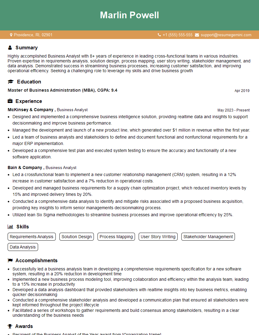
Interviews are opportunities to demonstrate your expertise, and this guide is here to help you shine. Explore the essential Data Analytics and Statistical Process Control interview questions that employers frequently ask, paired with strategies for crafting responses that set you apart from the competition.
Questions Asked in Data Analytics and Statistical Process Control Interview
Q 1. Explain the difference between descriptive, predictive, and prescriptive analytics.
Descriptive, predictive, and prescriptive analytics represent a progression in data analysis capabilities. Think of it like a journey from understanding the past to shaping the future.
- Descriptive Analytics: This is about summarizing and visualizing what has happened. It answers the ‘what’ questions. For example, analyzing sales data to determine the best-selling product over the last quarter. We use tools like dashboards and summary statistics (mean, median, mode) to understand past performance. Imagine reviewing a company’s sales report to see which product lines were most profitable last year; that’s descriptive analytics.
- Predictive Analytics: This focuses on forecasting what might happen in the future. It answers the ‘what if’ questions. Techniques like regression analysis, machine learning algorithms, and time series modeling are used. A classic example is predicting customer churn using past customer behavior data and machine learning models. Predictive analytics helps a bank anticipate potential loan defaults based on borrowers’ credit history.
- Prescriptive Analytics: This goes beyond prediction to recommend actions that optimize outcomes. It answers the ‘what should I do’ questions. It uses optimization techniques, simulation, and decision support systems. An example is using an algorithm to recommend the optimal pricing strategy to maximize profits, factoring in various market conditions. A supply chain optimization software suggesting the best routes for delivery based on real-time traffic and demand forecasts would be a prescriptive analytics application.
In essence, descriptive analytics describes the past, predictive analytics predicts the future, and prescriptive analytics prescribes the best course of action.
Q 2. Describe various types of control charts and their applications.
Control charts are powerful tools in Statistical Process Control (SPC) used to monitor process stability and identify potential problems. They visually display data over time, allowing us to quickly spot trends or deviations from the expected behavior.
- Shewhart Charts (X-bar and R charts): These are fundamental control charts used to monitor the average (X-bar) and range (R) of a process. The X-bar chart tracks the central tendency, while the R chart tracks the variability. They’re often used in manufacturing to monitor dimensions of parts or the weight of products.
- c-chart: This chart tracks the number of defects per unit. Think of inspecting a batch of t-shirts for flaws – each t-shirt is a unit, and the number of flaws on each is counted. Useful in quality control applications.
- u-chart: Similar to the c-chart, but it tracks the number of defects per unit, where the number of units inspected varies. For example, if you are inspecting different sized batches of cookies for the number of burnt ones.
- p-chart: Monitors the proportion of non-conforming units in a sample. For example, the percentage of defective light bulbs in a batch. Ideal for quality control where samples are examined for pass/fail criteria.
- Individuals and Moving Range (I-MR) charts: Used when data is collected individually, rather than in subgroups. For example, daily temperature readings. The I-chart tracks individual measurements, and the MR chart tracks the range between consecutive measurements.
The choice of control chart depends on the type of data being collected and the goals of the monitoring process. The charts provide immediate visual cues about process stability or instability and allow for timely intervention if problems are detected.
Q 3. What are the key assumptions of a linear regression model?
Linear regression models, while powerful, rely on several key assumptions. Violating these assumptions can lead to inaccurate and unreliable results. Let’s explore them:
- Linearity: There’s a linear relationship between the independent (predictor) and dependent (response) variables. A scatter plot can help assess this.
- Independence: Observations are independent of each other. Autocorrelation (correlation between observations over time) violates this assumption. For instance, stock prices are usually correlated over time, violating this assumption.
- Homoscedasticity: The variance of the errors (residuals) is constant across all levels of the independent variable. A plot of residuals vs. fitted values can detect heteroscedasticity (non-constant variance). Imagine the variability in house prices is much larger for expensive houses than for inexpensive houses.
- Normality: The errors (residuals) are normally distributed. A histogram or Q-Q plot of the residuals can be used to check this assumption.
- No or little Multicollinearity: Independent variables are not highly correlated with each other. High multicollinearity makes it difficult to isolate the individual effects of each predictor variable. Correlation matrices are commonly used to detect multicollinearity.
It’s important to check these assumptions after fitting a linear regression model using diagnostic plots and statistical tests. If assumptions are violated, transformations of variables or alternative modeling techniques may be necessary.
Q 4. How do you handle outliers in your dataset?
Outliers, data points that significantly deviate from the rest of the data, can heavily influence the results of statistical analyses. Handling them requires careful consideration. There’s no single ‘best’ method; the approach depends on the context and cause of the outlier.
- Identifying Outliers: Box plots, scatter plots, and Z-scores are common tools for identifying outliers. Z-scores measure how many standard deviations a data point is from the mean.
- Understanding the Cause: Is it a data entry error? A genuine extreme value? Investigating the cause is crucial. If it’s an error, correct it; if it’s genuine, consider whether it should be included in the analysis.
- Robust Methods: Using robust statistical methods like median instead of mean, or robust regression techniques, reduces the influence of outliers.
- Transformation: Transforming the data (e.g., using logarithms) can sometimes reduce the impact of outliers.
- Winsorizing or Trimming: Winsorizing replaces extreme values with less extreme values (e.g., replacing the highest value with the next highest). Trimming removes the extreme values altogether. Both these approaches reduce outlier influence but result in some data loss.
- Outlier removal (use with caution): Removing outliers is a last resort and should only be done after thorough investigation and justification. Always document why outliers were removed.
The key is to be transparent and justify your chosen method. Simply removing outliers without explanation is generally not acceptable.
Q 5. Explain the concept of statistical significance.
Statistical significance refers to the probability of observing a result as extreme as, or more extreme than, the one obtained if there were actually no effect (null hypothesis). It helps determine if an observed effect is likely due to chance or a real phenomenon.
We use p-values to assess statistical significance. A p-value is the probability of observing the data (or more extreme data) given that the null hypothesis is true. A small p-value (typically below 0.05) indicates that the observed result is unlikely to have occurred by chance alone, and we reject the null hypothesis. For instance, if we’re testing whether a new drug is effective, a small p-value suggests the observed improvement in symptoms is likely due to the drug and not just random chance.
It’s important to note that statistical significance does not necessarily imply practical significance. A statistically significant result might have a small effect size that’s not practically meaningful. Context and effect size are crucial in interpretation.
Q 6. What is the Central Limit Theorem and its importance in statistical inference?
The Central Limit Theorem (CLT) is a cornerstone of statistical inference. It states that the distribution of the sample means from a large number of independent random samples will approximate a normal distribution, regardless of the shape of the population distribution, as long as the population has a finite variance.
Importance in Statistical Inference: The CLT is crucial because many statistical tests assume normality. Even if the underlying population isn’t normally distributed, the CLT allows us to use these tests if we have a sufficiently large sample size. For example, if we want to estimate the average height of all adults, the CLT guarantees that the sample mean from a large sample will be normally distributed even if the distribution of heights in the population isn’t normal. This is why we can use t-tests (assuming normality of sample means) on many data sets, even if underlying data might not be normally distributed.
The larger the sample size, the closer the sampling distribution of the mean will be to a normal distribution. This is why the CLT is critical in building confidence intervals and performing hypothesis tests, facilitating inferences about population parameters based on sample data.
Q 7. Describe different methods for data cleaning and preprocessing.
Data cleaning and preprocessing are essential steps before any meaningful analysis can be performed. They involve handling missing values, outliers, inconsistencies, and transforming data into a suitable format. Imagine preparing ingredients before cooking a delicious meal.
- Handling Missing Values: This could involve imputation (filling in missing values using methods like mean, median, mode, or more sophisticated techniques like K-Nearest Neighbors), or removal of rows or columns with excessive missing data. The choice depends on the amount of missing data and the nature of the variable.
- Outlier Treatment: As discussed earlier, this could involve identification, investigation, transformation, or removal of outliers. The approach should be justified and documented.
- Data Transformation: This involves converting data into a more suitable format for analysis. Common transformations include standardization (z-score normalization), min-max scaling, log transformation, and one-hot encoding of categorical variables.
- Data Reduction: This reduces the dimensionality of the data, often using techniques like Principal Component Analysis (PCA) to handle high-dimensional datasets, improving computational efficiency and reducing noise.
- Data Consistency Checks: Identifying and correcting inconsistencies in data, such as misspellings, incorrect data types, or duplicate entries. This might involve using regular expressions or data validation rules.
- Feature Engineering: Creating new features from existing ones to enhance model performance. This could involve creating interaction terms, polynomial features, or date/time features.
The specific methods chosen depend on the dataset and the analysis goals. Thorough documentation of the preprocessing steps is critical for reproducibility and understanding the results.
Q 8. Explain the difference between Type I and Type II errors.
Type I and Type II errors are both potential mistakes in hypothesis testing. Think of it like a courtroom trial: we’re trying to determine if the defendant is guilty (our hypothesis).
A Type I error, also known as a false positive, occurs when we incorrectly reject a true null hypothesis. In our trial analogy, this is like convicting an innocent person. The probability of making a Type I error is denoted by alpha (α), often set at 0.05 (5%).
A Type II error, also known as a false negative, occurs when we fail to reject a false null hypothesis. In our trial, this is like letting a guilty person go free. The probability of making a Type II error is denoted by beta (β). The power of a test (1-β) represents the probability of correctly rejecting a false null hypothesis.
Example: Imagine testing a new drug. The null hypothesis is that the drug has no effect. A Type I error would be concluding the drug is effective when it’s not. A Type II error would be concluding the drug is ineffective when it actually is effective.
Q 9. How do you interpret a p-value?
The p-value is the probability of observing results as extreme as, or more extreme than, the results actually obtained, assuming the null hypothesis is true. It’s a measure of evidence against the null hypothesis.
A small p-value (typically less than 0.05) suggests strong evidence against the null hypothesis, leading us to reject it. However, it doesn’t prove the alternative hypothesis is true. A large p-value doesn’t necessarily mean the null hypothesis is true, only that there isn’t enough evidence to reject it.
Misinterpretations to avoid: The p-value is not the probability that the null hypothesis is true. It’s the probability of the data given the null hypothesis, not the other way around. Also, a p-value alone shouldn’t be the sole basis for decision-making; consider effect size and practical significance.
Example: If we get a p-value of 0.02 when testing if a new marketing campaign increased sales, we might conclude there’s enough evidence to suggest the campaign was effective (reject the null hypothesis of no effect).
Q 10. What is the difference between correlation and causation?
Correlation measures the strength and direction of a linear relationship between two variables. Causation implies that one variable directly influences or causes a change in another variable.
Correlation does not imply causation. Just because two variables are correlated doesn’t mean one causes the other. There could be a third, confounding variable influencing both.
Example: Ice cream sales and drowning incidents are positively correlated. This doesn’t mean ice cream causes drowning. Both are influenced by a third variable: hot weather.
To establish causation, we need to consider other factors, such as temporal precedence (cause precedes effect), a plausible mechanism, and ruling out alternative explanations. Experiments, particularly randomized controlled trials, are often the best way to investigate causal relationships.
Q 11. What are some common methods for feature selection?
Feature selection aims to identify the most relevant features (predictors) for a model, improving performance and reducing complexity. Common methods include:
- Filter methods: These use statistical measures (e.g., correlation, chi-squared test) to rank features independently of the model. They’re computationally efficient but may miss interactions between features.
- Wrapper methods: These use a model’s performance as a criterion to evaluate subsets of features. Examples include recursive feature elimination (RFE) and forward/backward selection. They’re more computationally expensive but can capture feature interactions.
- Embedded methods: These incorporate feature selection into the model training process itself. Regularization techniques like LASSO and Ridge regression add penalties to the model to shrink less important coefficients towards zero.
- Tree-based methods: Decision trees and random forests naturally rank feature importance based on their contribution to the model’s predictive accuracy.
The best method depends on the dataset, model, and computational resources. Often a combination of methods is employed.
Q 12. Explain the concept of A/B testing.
A/B testing is a randomized experiment used to compare two versions (A and B) of something – typically a website, app, or marketing campaign – to see which performs better. It’s a crucial technique for data-driven decision-making.
Participants are randomly assigned to either version A or version B. Key metrics are then measured and compared to determine which version leads to better outcomes. Statistical tests are used to assess the significance of the differences.
Example: A company might A/B test two different website layouts to see which one leads to a higher conversion rate (e.g., more purchases). One version (A) might have a simpler layout, while version B has more images and interactive elements. By randomly assigning users to each version and tracking conversions, the company can determine which layout is more effective.
Key elements: Randomization, control group (A), experimental group (B), clearly defined metrics, sufficient sample size, and appropriate statistical analysis.
Q 13. Describe different techniques for model evaluation and selection.
Model evaluation and selection aim to choose the best model for a given task. Techniques include:
- Metrics: Accuracy, precision, recall, F1-score (for classification); Mean Squared Error (MSE), Root Mean Squared Error (RMSE), R-squared (for regression). The choice depends on the problem and business context.
- Cross-validation: This technique splits the data into multiple folds, trains the model on some folds, and evaluates it on the remaining fold(s). This helps avoid overfitting and provides a more robust estimate of model performance.
- Train-test split: The data is divided into training and testing sets. The model is trained on the training set and evaluated on the unseen testing set.
- Hyperparameter tuning: This involves optimizing the model’s hyperparameters (parameters not learned from the data) to improve performance. Techniques include grid search, random search, and Bayesian optimization.
- Model selection criteria: AIC (Akaike Information Criterion) and BIC (Bayesian Information Criterion) can help compare models with different numbers of parameters, penalizing model complexity.
The process often involves iteratively evaluating different models using these techniques to select the one that best balances performance and simplicity.
Q 14. How do you handle missing data in your analysis?
Handling missing data is crucial for accurate analysis. Ignoring it can lead to biased results. Strategies include:
- Deletion: Removing rows or columns with missing values. Listwise deletion removes entire rows, while pairwise deletion uses available data for each analysis. Simple but can lead to information loss, especially with a lot of missing data.
- Imputation: Replacing missing values with estimated values. Methods include mean/median/mode imputation (simple but can distort distributions), k-Nearest Neighbors (k-NN) imputation (considers similar data points), and model-based imputation (uses a predictive model to estimate missing values).
- Multiple imputation: Creates multiple plausible imputed datasets and analyzes each one, combining the results to account for uncertainty in the imputation process.
The best approach depends on the amount and pattern of missing data, the mechanism of missingness (missing completely at random (MCAR), missing at random (MAR), missing not at random (MNAR)), and the impact on the analysis. Understanding the reasons for missing data is key. It’s often beneficial to explore patterns in missingness before choosing a strategy.
Q 15. What is the difference between supervised and unsupervised learning?
Supervised and unsupervised learning are two fundamental approaches in machine learning, differing primarily in how they use data to build models. Think of it like this: supervised learning is like having a teacher who provides labeled examples, while unsupervised learning is like exploring a dataset without a teacher, trying to discover patterns on your own.
Supervised Learning: In supervised learning, the algorithm is trained on a dataset where each data point is labeled with the correct answer (the ‘target’ or ‘dependent’ variable). The algorithm learns to map inputs to outputs based on these labeled examples. For instance, training a model to predict house prices (the target variable) based on features like size, location, and age. The model learns the relationship between the features and the price from the labeled data.
- Examples: Image classification (identifying cats vs. dogs), spam detection, credit risk assessment.
Unsupervised Learning: In contrast, unsupervised learning uses unlabeled data. The algorithm tries to discover inherent structure, patterns, or relationships within the data without any predefined target variable. Imagine a detective trying to solve a crime with only clues and no suspect profile – they’re uncovering patterns and connections to form a hypothesis.
- Examples: Customer segmentation, anomaly detection, dimensionality reduction.
In short: supervised learning predicts, while unsupervised learning describes.
Career Expert Tips:
- Ace those interviews! Prepare effectively by reviewing the Top 50 Most Common Interview Questions on ResumeGemini.
- Navigate your job search with confidence! Explore a wide range of Career Tips on ResumeGemini. Learn about common challenges and recommendations to overcome them.
- Craft the perfect resume! Master the Art of Resume Writing with ResumeGemini’s guide. Showcase your unique qualifications and achievements effectively.
- Don’t miss out on holiday savings! Build your dream resume with ResumeGemini’s ATS optimized templates.
Q 16. Explain the concept of overfitting and how to avoid it.
Overfitting occurs when a model learns the training data too well, capturing noise and random fluctuations instead of the underlying patterns. This leads to excellent performance on the training data but poor generalization to unseen data. Think of a student memorizing the answers to a specific test without truly understanding the subject matter; they’ll ace that test, but fail any other assessment.
How to Avoid Overfitting:
- More Data: The simplest and often most effective method. More data provides a more robust representation of the underlying patterns.
- Cross-Validation: This technique divides the data into multiple subsets, training the model on some subsets and validating it on others. This helps assess how well the model generalizes.
- Feature Selection/Engineering: Carefully selecting or creating relevant features reduces the model’s complexity and avoids overfitting on irrelevant information. Removing noisy or redundant features is crucial.
- Regularization Techniques: Techniques like L1 (LASSO) and L2 (Ridge) regularization add penalties to the model’s complexity, discouraging it from fitting the noise.
- Early Stopping: In iterative models, stopping training before the model has fully converged on the training data can prevent overfitting.
- Pruning (for decision trees): Removing branches of a decision tree that don’t significantly improve accuracy helps prevent overfitting.
By employing these strategies, you can build a model that generalizes well to new, unseen data and provides reliable predictions.
Q 17. What are some common metrics used to evaluate classification models?
Evaluating classification models involves assessing their ability to correctly classify data points into different categories. Common metrics include:
- Accuracy: The ratio of correctly classified instances to the total number of instances. Simple, but can be misleading with imbalanced datasets.
- Precision: Out of all the instances predicted as positive, what proportion was actually positive? Useful when the cost of false positives is high (e.g., incorrectly identifying someone as having a disease).
- Recall (Sensitivity): Out of all the actual positive instances, what proportion was correctly identified? Important when the cost of false negatives is high (e.g., missing a disease diagnosis).
- F1-Score: The harmonic mean of precision and recall, providing a balanced measure of both. Useful when both false positives and false negatives are important.
- AUC-ROC (Area Under the Receiver Operating Characteristic curve): Measures the model’s ability to distinguish between classes across different thresholds. A higher AUC indicates better performance.
- Confusion Matrix: A table showing the counts of true positives, true negatives, false positives, and false negatives. Provides a detailed breakdown of the model’s performance.
The choice of metric depends on the specific problem and the relative costs of different types of errors.
Q 18. What are some common metrics used to evaluate regression models?
Regression models predict a continuous target variable. Evaluating their performance requires metrics that quantify the difference between predicted and actual values. Common metrics include:
- Mean Squared Error (MSE): The average of the squared differences between predicted and actual values. Sensitive to outliers.
- Root Mean Squared Error (RMSE): The square root of the MSE. Easier to interpret than MSE as it’s in the same units as the target variable.
- Mean Absolute Error (MAE): The average of the absolute differences between predicted and actual values. Less sensitive to outliers than MSE.
- R-squared (R²): Represents the proportion of variance in the target variable explained by the model. Ranges from 0 to 1, with higher values indicating better fit. However, a high R² doesn’t automatically imply a good model; it can be inflated by overfitting.
- Adjusted R-squared: A modified version of R² that adjusts for the number of predictors in the model, penalizing the inclusion of irrelevant variables.
Selecting the appropriate metric depends on the context of the problem and the desired emphasis on different types of errors. For instance, in finance, RMSE might be preferred because of its sensitivity to large errors.
Q 19. Explain the concept of process capability analysis.
Process capability analysis determines if a process is capable of consistently producing outputs that meet predefined specifications. It’s like assessing whether a factory’s machines consistently produce products within the required tolerances. We assess the process’s natural variability against the customer’s requirements (specifications).
The analysis typically involves calculating capability indices, such as:
- Cp (Process Capability Index): Measures the ratio of the specification width to the process spread (6 standard deviations). Indicates the inherent capability of the process, irrespective of its centering.
- Cpk (Process Capability Index): Considers both the process spread and its centering relative to the specification limits. A more realistic measure as it accounts for process centering.
These indices provide a numerical assessment of the process capability. A Cp or Cpk value greater than 1 typically indicates that the process is capable of meeting the specifications.
Example: Imagine a manufacturer producing bolts with a specified diameter of 10mm ± 0.1mm. Process capability analysis would determine if the manufacturing process consistently produces bolts within this range.
Q 20. Describe different methods for monitoring process stability.
Monitoring process stability involves tracking the process’s behavior over time to detect any shifts or changes that might indicate instability. This is critical for maintaining consistent quality and preventing defects.
Common methods include:
- Control Charts: These are graphical tools used to monitor process variables over time. Common types include X-bar and R charts (for continuous data), p-charts (for proportions), and c-charts (for counts). Control charts display data points alongside control limits; points outside the limits signal potential instability.
- Time Series Analysis: Statistical methods to identify trends, seasonality, and other patterns in process data over time. Can reveal gradual shifts or cyclical variations.
- Run Charts: Simpler than control charts; they plot data points over time without control limits. Useful for initial assessment of process stability.
- Statistical Process Control (SPC) Software: Automated tools that simplify control chart construction, analysis, and interpretation. These tools often incorporate advanced techniques for detecting subtle shifts in the process.
The choice of method depends on the type of data and the specific needs of the process. Control charts are very popular for their visual clarity and ability to quickly detect out-of-control conditions.
Q 21. How do you identify and address special cause variation?
Special cause variation refers to unpredictable, assignable variation in a process caused by specific, identifiable factors. It’s like a sudden hiccup in an otherwise smooth process, unlike common cause variation which is inherent to the process. Identifying and addressing special cause variation is crucial for process improvement.
Identifying Special Cause Variation:
- Control Charts: Points outside the control limits or non-random patterns (e.g., trends, runs) on a control chart strongly suggest special cause variation.
- Process Data Analysis: Investigate unusual data points or trends to pinpoint potential causes. This might involve examining process logs, operator reports, or equipment maintenance records.
- Root Cause Analysis (RCA): Techniques like the 5 Whys or fishbone diagrams to systematically identify the root causes of the variation.
Addressing Special Cause Variation:
- Investigate and Correct: Once a special cause is identified, take corrective action to eliminate it. This might involve repairing equipment, retraining personnel, changing materials, or improving a process step.
- Prevent Recurrence: Implement measures to prevent the special cause from recurring. This might involve better process controls, preventive maintenance, or improved training.
- Document Findings: Record the identified special cause, the corrective action taken, and the results. This helps prevent similar issues in the future.
Effective identification and addressing of special cause variation leads to a more stable and predictable process, ultimately resulting in improved quality and reduced costs.
Q 22. What are the steps involved in implementing a Six Sigma project?
Implementing a Six Sigma project follows a structured DMAIC methodology: Define, Measure, Analyze, Improve, and Control.
- Define: Clearly define the project’s goals, scope, and customer requirements. This involves identifying the critical-to-quality (CTQ) characteristics and setting measurable targets. For example, reducing customer complaints related to late order delivery.
- Measure: Collect data to understand the current process performance. This includes identifying key performance indicators (KPIs) and using appropriate statistical tools to measure process capability. This might involve analyzing the current average delivery time and its standard deviation.
- Analyze: Identify the root causes of defects or variations in the process. This step utilizes various statistical tools like Pareto charts, fishbone diagrams, and regression analysis to pinpoint the key factors contributing to the problem. For example, identifying bottlenecks in the order processing system as a major contributor to late deliveries.
- Improve: Develop and implement solutions to address the root causes identified in the analysis phase. This could involve process redesign, training, or new technology implementation. For example, implementing a new order management system or optimizing warehouse logistics.
- Control: Establish monitoring systems to ensure that the improvements are sustained. This involves setting up control charts and regularly tracking KPIs to prevent regression to the previous state. For example, regularly monitoring delivery times and investigating any deviations from the established target.
Each phase involves iterative problem-solving and data-driven decision making. The success of a Six Sigma project hinges on strong data analysis and a systematic approach.
Q 23. Explain the concept of control limits.
Control limits in statistical process control (SPC) are boundaries on a control chart that help determine if a process is stable and predictable. They are calculated based on the process data and represent the expected variation in the process under normal operating conditions.
There are three main types of control limits:
- Upper Control Limit (UCL): The upper boundary of the control chart. Points exceeding the UCL suggest a possible special cause of variation, indicating that the process is out of control.
- Central Line (CL): The average of the process data. It represents the mean of the process.
- Lower Control Limit (LCL): The lower boundary of the control chart. Points below the LCL also indicate a possible special cause of variation, suggesting the process is out of control.
Control limits are crucial for identifying shifts or changes in the process that might lead to defects or non-conforming products. They are not the same as specification limits, which define the acceptable range for the product or service characteristics.
Imagine a control chart for the weight of candy bars produced in a factory. The control limits will define the acceptable range of variation in weight. If a point falls outside these limits, it indicates that something unusual happened during the production process (maybe a machine malfunction), requiring investigation.
Q 24. How do you determine the sample size for a statistical study?
Determining the appropriate sample size for a statistical study is critical to ensure the results are reliable and meaningful. It depends on several factors:
- Desired level of precision: How much error are you willing to tolerate in your estimates? A smaller margin of error requires a larger sample size.
- Confidence level: How confident do you want to be that your results reflect the true population value? A higher confidence level (e.g., 99% instead of 95%) requires a larger sample size.
- Population variability: The more variable the data, the larger the sample size needed to obtain a precise estimate.
- Population size: For very large populations, the sample size can be relatively small while still providing accurate results. For small populations, a larger proportion of the population may need to be sampled.
There are formulas and online calculators that can help determine the required sample size, often utilizing the ‘Z-score’ corresponding to the desired confidence level and the expected margin of error. For example, if we’re conducting a survey and want to estimate the proportion of people who prefer a certain product with a 5% margin of error and 95% confidence, the appropriate sample size calculation would consider these factors.
In practice, it’s often beneficial to conduct a pilot study with a smaller sample size to get a preliminary estimate of the population variance and refine the sample size calculation for the main study.
Q 25. What are some common software tools used for data analysis and statistical process control?
Many software tools are used for data analysis and statistical process control. Here are some common examples:
- R: A powerful open-source programming language and environment for statistical computing and graphics. It’s highly versatile and offers a wide range of packages for SPC and other data analysis tasks.
- Python (with libraries like Pandas, NumPy, SciPy, Statsmodels): Python, combined with these powerful libraries, provides an excellent platform for data manipulation, statistical analysis, and visualization. Its flexibility and extensive community support make it a popular choice.
- Minitab: A dedicated statistical software package widely used in industry for quality control and Six Sigma projects. It provides user-friendly tools for SPC, hypothesis testing, and design of experiments.
- JMP: Another commercially available statistical software package known for its interactive graphical interface and powerful data visualization capabilities. It’s well-suited for exploratory data analysis and process improvement projects.
- Microsoft Excel (with Data Analysis Toolpak): While not as powerful as dedicated statistical packages, Excel offers basic statistical functions and the Data Analysis Toolpak, which provides additional tools for hypothesis testing and regression analysis. It is suitable for simpler analyses.
The best choice depends on the specific needs of the analysis, the user’s expertise, and available resources.
Q 26. Describe your experience with hypothesis testing.
Hypothesis testing is a crucial part of statistical inference. It involves formulating a hypothesis about a population parameter (e.g., the mean, proportion) and then using sample data to determine whether there is enough evidence to reject the null hypothesis in favor of an alternative hypothesis.
The process typically involves these steps:
- State the hypotheses: Define the null hypothesis (H0), which represents the status quo, and the alternative hypothesis (H1 or Ha), which represents the claim we’re trying to support.
- Set the significance level (alpha): This is the probability of rejecting the null hypothesis when it’s actually true (Type I error). A common value is 0.05.
- Choose the appropriate test statistic: This depends on the type of data (e.g., t-test for means, z-test for proportions, chi-squared test for categorical data).
- Collect data and calculate the test statistic: Use the sample data to calculate the value of the test statistic.
- Determine the p-value: This is the probability of observing the obtained results or more extreme results, assuming the null hypothesis is true. A small p-value (typically less than alpha) provides evidence to reject the null hypothesis.
- Make a decision: If the p-value is less than alpha, reject the null hypothesis; otherwise, fail to reject the null hypothesis.
For example, I once used a t-test to determine if a new marketing campaign significantly increased sales compared to the previous campaign. The null hypothesis was that there was no difference in sales, and the alternative hypothesis was that the new campaign increased sales. The p-value from the t-test allowed me to determine whether to reject the null hypothesis and conclude that the new campaign was effective.
Q 27. Explain your understanding of different probability distributions.
Probability distributions describe the likelihood of different outcomes in a random process. Several common distributions are crucial in data analysis and statistical process control.
- Normal distribution: A symmetric, bell-shaped distribution characterized by its mean and standard deviation. Many natural phenomena follow this distribution approximately, making it fundamental in statistical inference.
- Binomial distribution: Describes the probability of getting a certain number of successes in a fixed number of independent Bernoulli trials (experiments with only two outcomes, like success or failure). Used for modeling count data.
- Poisson distribution: Describes the probability of a given number of events occurring in a fixed interval of time or space, when these events are independent and occur with a constant average rate. Used for modeling rare events.
- Exponential distribution: Describes the time between events in a Poisson process. Often used for modeling the time until failure of a system or component.
- Chi-squared distribution: Used in hypothesis testing related to variances and goodness-of-fit tests for categorical data.
- t-distribution: Similar to the normal distribution but with heavier tails; used for hypothesis testing when the population standard deviation is unknown.
- F-distribution: Used in analysis of variance (ANOVA) to compare the variances of two or more groups.
Understanding these distributions allows us to model data appropriately, make inferences about populations, and assess the reliability of statistical results.
Q 28. Describe a situation where you used statistical analysis to solve a real-world problem.
In a previous role, I worked with a manufacturing company experiencing high rates of defects in their production process. We suspected that the variation in temperature during the manufacturing process was a contributing factor.
Using statistical process control techniques, specifically control charts, I analyzed data collected on the temperature and the number of defects produced at various temperature levels. I discovered that temperature fluctuations outside a specific range strongly correlated with an increased defect rate. This analysis revealed a clear pattern and allowed us to identify specific time periods and temperature levels associated with higher defects.
This evidence led to improvements in the temperature control system, resulting in a significant reduction in the defect rate and a substantial cost savings for the company. This involved careful data collection, implementing appropriate statistical tests, interpreting the results, and effectively communicating them to stakeholders to achieve a practical solution.
Key Topics to Learn for Data Analytics and Statistical Process Control Interview
- Descriptive Statistics: Understanding measures of central tendency (mean, median, mode), dispersion (variance, standard deviation), and their interpretations. Practical application: Analyzing key performance indicators (KPIs) to identify trends and areas for improvement.
- Inferential Statistics: Hypothesis testing, confidence intervals, and regression analysis. Practical application: Determining the statistical significance of findings and making data-driven decisions.
- Control Charts (SPC): Understanding different types of control charts (e.g., X-bar and R charts, p-charts, c-charts) and their applications in monitoring process stability. Practical application: Identifying and addressing process variations to improve quality and efficiency.
- Data Visualization: Creating effective charts and graphs to communicate data insights clearly. Practical application: Presenting analytical findings to stakeholders in a compelling and understandable manner.
- Data Cleaning and Preprocessing: Handling missing data, outliers, and inconsistencies in datasets. Practical application: Ensuring data quality and accuracy for reliable analysis.
- Process Capability Analysis: Assessing the ability of a process to meet specifications. Practical application: Determining if a process is capable of producing products or services that meet customer requirements.
- Statistical Software Proficiency: Demonstrating familiarity with statistical software packages like R, Python (with libraries like Pandas and Scikit-learn), or SAS. Practical application: Efficiently performing complex statistical analyses and generating reports.
- Problem-Solving and Critical Thinking: Applying statistical concepts to solve real-world problems and critically evaluating data and results. Practical application: Formulating data-driven solutions to business challenges.
Next Steps
Mastering Data Analytics and Statistical Process Control opens doors to exciting and rewarding careers in various industries. These skills are highly sought after, leading to increased job opportunities and higher earning potential. To maximize your chances of landing your dream role, crafting a strong, ATS-friendly resume is crucial. ResumeGemini is a trusted resource that can help you build a professional and impactful resume, ensuring your qualifications shine. Examples of resumes tailored to Data Analytics and Statistical Process Control are available to guide you. Take the next step towards your successful career journey today!
Explore more articles
Users Rating of Our Blogs
Share Your Experience
We value your feedback! Please rate our content and share your thoughts (optional).
What Readers Say About Our Blog
Hello,
We found issues with your domain’s email setup that may be sending your messages to spam or blocking them completely. InboxShield Mini shows you how to fix it in minutes — no tech skills required.
Scan your domain now for details: https://inboxshield-mini.com/
— Adam @ InboxShield Mini
Reply STOP to unsubscribe
Hi, are you owner of interviewgemini.com? What if I told you I could help you find extra time in your schedule, reconnect with leads you didn’t even realize you missed, and bring in more “I want to work with you” conversations, without increasing your ad spend or hiring a full-time employee?
All with a flexible, budget-friendly service that could easily pay for itself. Sounds good?
Would it be nice to jump on a quick 10-minute call so I can show you exactly how we make this work?
Best,
Hapei
Marketing Director
Hey, I know you’re the owner of interviewgemini.com. I’ll be quick.
Fundraising for your business is tough and time-consuming. We make it easier by guaranteeing two private investor meetings each month, for six months. No demos, no pitch events – just direct introductions to active investors matched to your startup.
If youR17;re raising, this could help you build real momentum. Want me to send more info?
Hi, I represent an SEO company that specialises in getting you AI citations and higher rankings on Google. I’d like to offer you a 100% free SEO audit for your website. Would you be interested?
Hi, I represent an SEO company that specialises in getting you AI citations and higher rankings on Google. I’d like to offer you a 100% free SEO audit for your website. Would you be interested?
good
