Cracking a skill-specific interview, like one for Statistical Software (e.g., Minitab, R), requires understanding the nuances of the role. In this blog, we present the questions you’re most likely to encounter, along with insights into how to answer them effectively. Let’s ensure you’re ready to make a strong impression.
Questions Asked in Statistical Software (e.g., Minitab, R) Interview
Q 1. Explain the difference between a Type I and Type II error.
Type I and Type II errors are both errors in statistical hypothesis testing. They represent different ways we can be wrong when making a decision about a hypothesis. Think of it like a medical test: we’re trying to determine if someone has a disease.
Type I Error (False Positive): This occurs when we reject the null hypothesis when it is actually true. In our medical analogy, this is saying someone has the disease when they actually don’t. The probability of making a Type I error is denoted by α (alpha), often set at 0.05 (5%).
Type II Error (False Negative): This occurs when we fail to reject the null hypothesis when it is actually false. In our medical example, this means saying someone doesn’t have the disease when they actually do. The probability of making a Type II error is denoted by β (beta). The power of a test (1 – β) represents the probability of correctly rejecting a false null hypothesis.
Example: Imagine testing a new drug. The null hypothesis is that the drug has no effect. A Type I error would be concluding the drug is effective when it’s not. A Type II error would be concluding the drug is ineffective when it actually is effective.
Q 2. Describe the central limit theorem.
The Central Limit Theorem (CLT) is a fundamental concept in statistics. It states that the distribution of the sample means of a large number of independent, identically distributed random variables, regardless of their original distribution, will approximate a normal distribution. This is true even if the original data isn’t normally distributed!
In simpler terms: Imagine you’re taking many samples from a population (e.g., measuring the heights of people). If you calculate the average height for each sample and plot those averages, the resulting distribution will look like a bell curve (normal distribution), even if the original heights weren’t normally distributed. The larger your sample size, the closer this approximation will be to a perfect normal distribution.
Importance: The CLT is crucial because it allows us to use the normal distribution to make inferences about population parameters (like the mean) even when we don’t know the true distribution of the population. This is widely used in hypothesis testing and confidence interval construction.
Q 3. What are the assumptions of linear regression?
Linear regression models the relationship between a dependent variable and one or more independent variables. Several assumptions underpin its validity and accurate interpretation:
- Linearity: There’s a linear relationship between the dependent and independent variables. A scatter plot can help visually assess this.
- Independence of errors: The errors (residuals) are independent of each other. Autocorrelation violates this assumption.
- Homoscedasticity: The variance of the errors is constant across all levels of the independent variable(s). This means the spread of the residuals should be roughly the same for all predicted values.
- Normality of errors: The errors are normally distributed. This assumption is particularly important for small sample sizes and for making inferences about individual regression coefficients.
- No multicollinearity (for multiple linear regression): Independent variables should not be highly correlated with each other. High multicollinearity can inflate standard errors and make it difficult to interpret the individual effects of predictors.
- No significant outliers: Outliers can disproportionately influence the regression line.
Checking Assumptions: Software like Minitab and R provide diagnostic tools (residual plots, normality tests, etc.) to check these assumptions. If assumptions are violated, transformations of variables or alternative modeling techniques might be necessary.
Q 4. How do you handle missing data in a dataset?
Missing data is a common challenge in data analysis. The best approach depends on the nature and extent of the missing data, as well as the research question. There’s no one-size-fits-all solution.
- Deletion Methods:
- Listwise deletion (complete case analysis): Remove any rows with missing values. Simple but can lead to significant loss of information if missingness is not random.
- Pairwise deletion: Use all available data for each analysis, even if some cases have missing values on some variables. This can lead to inconsistencies.
- Imputation Methods:
- Mean/median/mode imputation: Replace missing values with the mean, median, or mode of the observed values. Simple but can underestimate variability.
- Regression imputation: Predict missing values using a regression model based on other variables. More sophisticated but assumes a linear relationship.
- Multiple imputation: Create multiple plausible imputed datasets and analyze each separately, combining the results. A more robust method that accounts for uncertainty in imputed values.
Choosing a method: The choice depends on the pattern of missing data (missing completely at random (MCAR), missing at random (MAR), missing not at random (MNAR)). If missingness is not MCAR, imputation methods are generally preferred over deletion.
Q 5. What are the strengths and weaknesses of using R for data analysis?
R is a powerful and versatile open-source statistical computing environment with many strengths, but also some drawbacks:
Strengths:
- Open-source and free: Accessible to everyone.
- Extensive libraries: CRAN (Comprehensive R Archive Network) provides a vast collection of packages for various statistical methods and data visualization.
- Flexibility and customization: R allows for highly customized analyses and visualizations.
- Large and active community: Abundant online resources, tutorials, and support.
- Reproducibility: R scripts can be easily shared and reproduced.
Weaknesses:
- Steeper learning curve: Requires programming skills.
- Syntax can be challenging: Can be less intuitive than point-and-click software.
- Data management can be cumbersome: Requires more effort for data cleaning and manipulation compared to user-friendly interfaces.
- Debugging can be difficult: Identifying and fixing errors in R code can be time-consuming.
Q 6. What are the strengths and weaknesses of using Minitab for statistical analysis?
Minitab is a user-friendly commercial statistical software package with its own set of advantages and disadvantages:
Strengths:
- User-friendly interface: Point-and-click interface makes it easy to use, even for users without extensive statistical knowledge.
- Comprehensive statistical capabilities: Offers a wide range of statistical tools and techniques.
- Clear and concise output: Provides well-organized and easy-to-interpret results.
- Good for teaching and learning: Its simplicity makes it suitable for introductory statistics courses.
- Excellent graphical capabilities: Generates high-quality graphs and charts.
Weaknesses:
- Cost: It’s a commercial software, so it’s not free.
- Limited customization: Less flexibility than R for advanced users.
- Automation capabilities are limited compared to R: Complex workflows may require more manual steps.
- Relatively smaller community: Compared to R, the community support is smaller.
Q 7. Explain the concept of p-value.
The p-value is a probability that measures the strength of evidence against a null hypothesis. It represents the probability of observing results as extreme as, or more extreme than, the ones obtained, assuming the null hypothesis is true.
In simpler terms: Imagine you’re flipping a coin 10 times and getting 9 heads. The null hypothesis is that the coin is fair (50% chance of heads). The p-value would tell you the probability of getting 9 or more heads if the coin were actually fair. A small p-value suggests that the observed results are unlikely under the null hypothesis, providing evidence against it.
Interpreting p-values: A commonly used threshold is 0.05. If the p-value is less than 0.05, the null hypothesis is typically rejected (statistically significant). However, the p-value should be interpreted in the context of the study design, sample size, and practical significance. A small p-value doesn’t automatically mean the effect is large or important in the real world.
Important Note: The p-value is not the probability that the null hypothesis is true. It’s the probability of observing the data given the null hypothesis is true.
Q 8. What is the difference between correlation and causation?
Correlation and causation are often confused, but they are distinct concepts. Correlation describes a relationship between two variables; as one changes, the other tends to change as well. Causation, on the other hand, implies that one variable directly influences or causes a change in another. Just because two things are correlated doesn’t mean one causes the other.
Example: Ice cream sales and drowning incidents are often positively correlated – both increase in the summer. However, eating ice cream doesn’t cause drowning. The underlying cause is the warm weather, which leads to more people swimming and buying ice cream. This is a classic example of spurious correlation.
In statistical software like R or Minitab, you can calculate correlation using functions like cor() in R or the Correlation command in Minitab. However, correlation analysis alone cannot establish causation. To determine causation, you need to consider other factors and often employ more rigorous methods like controlled experiments or causal inference techniques.
Q 9. Describe different methods for outlier detection.
Outlier detection is crucial for data cleaning and accurate analysis. Outliers are data points significantly different from other observations. Several methods exist:
- Visual Inspection: Creating scatter plots, box plots, or histograms can visually reveal outliers. This is a quick and intuitive first step.
- Z-score method: Calculates how many standard deviations a data point is from the mean. Data points with a Z-score exceeding a threshold (e.g., ±3) are often considered outliers. This is easily implemented in R using
scale()or in Minitab using the descriptive statistics function. - Interquartile Range (IQR) method: This method uses the difference between the 75th percentile (Q3) and the 25th percentile (Q1) of the data. Data points outside the range Q1 – 1.5*IQR and Q3 + 1.5*IQR are potential outliers.
- DBSCAN (Density-Based Spatial Clustering of Applications with Noise): A clustering algorithm that identifies outliers as points with low density compared to their neighbors. This is particularly useful for high-dimensional data. R packages like
dbscanprovide easy implementation.
The choice of method depends on the data’s nature and the specific analysis goals. It’s often beneficial to use multiple methods to gain a comprehensive understanding of potential outliers.
Q 10. Explain different methods for data normalization.
Data normalization scales data to a specific range, often between 0 and 1 or -1 and 1. This is essential for many machine learning algorithms and statistical methods which are sensitive to feature scaling. Common normalization methods include:
- Min-Max scaling: Scales data to a range between 0 and 1. The formula is:
(x - min(x)) / (max(x) - min(x)). This is easily implemented in R using thescale()function with thecenter = FALSEandscale = TRUEarguments. Minitab offers similar functionalities. - Z-score normalization (Standardization): Transforms data to have a mean of 0 and a standard deviation of 1. The formula is:
(x - mean(x)) / sd(x). In R, this is done usingscale()(default settings). Minitab also provides a built-in standardization process. - Robust scaling: Uses the median and interquartile range (IQR) instead of the mean and standard deviation, making it less sensitive to outliers. R packages such as
robustbaseprovide functions for this.
The best method depends on the data distribution and the intended use. Min-Max scaling is preferred when the data is approximately uniformly distributed. Z-score normalization is more appropriate for normally distributed data. Robust scaling handles outliers better than Min-Max and Z-score.
Q 11. How do you perform hypothesis testing?
Hypothesis testing is a formal procedure for making decisions about a population based on sample data. It involves formulating a null hypothesis (H0), which is a statement of no effect or no difference, and an alternative hypothesis (H1), which is the statement we want to support.
Steps:
- State the hypotheses: Define H0 and H1 clearly.
- Choose a significance level (α): This is the probability of rejecting H0 when it is true (Type I error). Common values are 0.05 or 0.01.
- Select a test statistic: The choice depends on the data type and the hypotheses (e.g., t-test, z-test, chi-square test, ANOVA). Many statistical software packages have built-in functions for various tests (R:
t.test(),chisq.test(); Minitab: various options in the ‘Stat’ menu). - Calculate the test statistic and p-value: The p-value is the probability of observing the obtained results (or more extreme results) if H0 were true.
- Make a decision: If the p-value is less than α, reject H0; otherwise, fail to reject H0.
Example: Testing if a new drug lowers blood pressure. H0: The drug has no effect. H1: The drug lowers blood pressure. A t-test would be appropriate. If the p-value is less than 0.05, we reject H0 and conclude that the drug is effective.
Q 12. What are confidence intervals and how are they calculated?
Confidence intervals provide a range of plausible values for a population parameter (e.g., mean, proportion) based on sample data. They quantify the uncertainty associated with estimating the parameter.
A 95% confidence interval, for example, means that if we were to repeat the sampling process many times, 95% of the calculated intervals would contain the true population parameter.
Calculation (for a population mean):
The formula for a confidence interval for the population mean is:
[sample mean - (critical value * standard error), sample mean + (critical value * standard error)]
Where:
- Sample mean is the average of the sample data.
- Critical value is determined by the desired confidence level and the sample size (often obtained from a t-distribution table or calculated using statistical software).
- Standard error is the standard deviation of the sample mean, calculated as
sample standard deviation / sqrt(sample size).
Both R (using the t.test() function) and Minitab provide straightforward ways to calculate confidence intervals.
Q 13. Explain different regression techniques (linear, logistic, etc.).
Regression techniques model the relationship between a dependent variable and one or more independent variables. Different types exist depending on the nature of the dependent variable:
- Linear Regression: Models the relationship between a continuous dependent variable and one or more independent variables using a linear equation. Assumes a linear relationship between variables. Implemented in R using
lm()and in Minitab using the Regression command. - Logistic Regression: Models the relationship between a binary (0/1) dependent variable and one or more independent variables. Predicts the probability of the dependent variable being 1. R:
glm()withfamily = binomial; Minitab: Logistic Regression command. - Polynomial Regression: Models non-linear relationships by including polynomial terms of the independent variables in the regression equation. Useful for capturing curved relationships. In R, you can achieve this by adding polynomial terms manually in the
lm()formula. - Multiple Linear Regression: Extends linear regression to handle multiple independent variables. R and Minitab offer the same commands for this extension.
Choosing the appropriate regression technique depends on the nature of the data and the research question. Assumptions like linearity, normality, and independence of errors need to be checked before interpreting the results.
Q 14. Describe various data visualization techniques and their applications.
Data visualization is crucial for exploring, understanding, and communicating data insights. Various techniques exist:
- Histograms: Show the frequency distribution of a continuous variable.
- Scatter plots: Display the relationship between two continuous variables.
- Box plots: Show the distribution of a variable, including quartiles, median, and outliers.
- Bar charts: Compare the frequencies or means of different categories.
- Line charts: Show trends over time or across categories.
- Heatmaps: Visualize correlation matrices or other tabular data using color intensity.
- Pie charts: Show proportions of different categories.
Applications:
- Exploratory data analysis (EDA): Identify patterns, trends, and outliers.
- Presentation of findings: Communicate insights effectively to stakeholders.
- Model diagnostics: Assess the assumptions and performance of statistical models (e.g., residual plots in regression).
R (using ggplot2) and Minitab offer a wide range of tools for creating various data visualizations. The choice of visualization method depends on the data type and the message one wants to convey.
Q 15. How do you choose the appropriate statistical test for a given dataset?
Choosing the right statistical test depends entirely on your research question, the type of data you have, and the assumptions you can make about that data. It’s like choosing the right tool for a job – you wouldn’t use a hammer to screw in a screw!
First, identify your data type: Is it categorical (e.g., colors, types of fruit) or numerical (e.g., height, weight)? Then, determine your research question: Are you comparing groups, looking for correlations, or predicting an outcome?
- Comparing groups (categorical outcome): Chi-square test (for categorical data), Fisher’s exact test (for small sample sizes), or t-tests/ANOVA (if the outcome is ordinal and can be treated as numerical).
- Comparing groups (numerical outcome): Independent samples t-test (two groups), paired samples t-test (repeated measures on the same group), ANOVA (three or more groups).
- Correlation: Pearson correlation (linear relationship between two numerical variables), Spearman correlation (monotonic relationship between two variables, doesn’t require normality), Kendall’s tau (another non-parametric correlation measure).
- Prediction (regression): Linear regression (predicting a numerical outcome), logistic regression (predicting a categorical outcome).
Consider the assumptions of each test (e.g., normality, independence of observations). Violating assumptions can lead to inaccurate results. Software like R or Minitab can help check these assumptions and suggest appropriate tests.
Example: Imagine you’re comparing the average heights of men and women. You have numerical height data and two groups (men and women). An independent samples t-test would be appropriate if the data is approximately normally distributed. If not, you might consider a non-parametric alternative like the Mann-Whitney U test.
Career Expert Tips:
- Ace those interviews! Prepare effectively by reviewing the Top 50 Most Common Interview Questions on ResumeGemini.
- Navigate your job search with confidence! Explore a wide range of Career Tips on ResumeGemini. Learn about common challenges and recommendations to overcome them.
- Craft the perfect resume! Master the Art of Resume Writing with ResumeGemini’s guide. Showcase your unique qualifications and achievements effectively.
- Don’t miss out on holiday savings! Build your dream resume with ResumeGemini’s ATS optimized templates.
Q 16. Explain ANOVA (Analysis of Variance).
ANOVA, or Analysis of Variance, is a statistical test used to compare the means of three or more groups. Think of it as an extension of the t-test, which only compares two means. ANOVA determines if there are statistically significant differences between the means of these groups, or if the observed differences are likely due to random chance.
ANOVA works by partitioning the total variation in the data into different sources of variation:
- Between-group variation: The variation between the means of the different groups.
- Within-group variation: The variation within each group.
ANOVA calculates an F-statistic, which is the ratio of between-group variation to within-group variation. A large F-statistic suggests that the between-group variation is significantly larger than the within-group variation, indicating that there are likely differences between the group means.
There are different types of ANOVA: One-way ANOVA (comparing groups based on one factor), two-way ANOVA (comparing groups based on two factors), and repeated measures ANOVA (comparing groups based on repeated measurements on the same subjects).
Example: You want to compare the effectiveness of three different fertilizers on crop yield. You could use a one-way ANOVA to test if there’s a statistically significant difference in yield among the three fertilizer groups. The results will indicate whether the fertilizers have different effects on crop yields or not.
Q 17. What is a box plot and how is it used in data analysis?
A box plot, also known as a box-and-whisker plot, is a graphical representation of the distribution of a dataset. It visually displays the median, quartiles, and outliers of the data. Imagine it as a summary snapshot of your data’s spread and central tendency.
The box represents the interquartile range (IQR), which is the range between the first quartile (25th percentile) and the third quartile (75th percentile). The line inside the box represents the median (50th percentile). The whiskers extending from the box typically represent the range of the data, excluding outliers. Outliers are usually plotted as individual points beyond the whiskers.
Uses in data analysis:
- Identifying outliers: Box plots clearly highlight potential outliers, which could be errors or genuinely unusual data points requiring further investigation.
- Comparing distributions: By plotting box plots for different groups side-by-side, you can easily compare their central tendencies and spreads. This is particularly useful for visualizing the results of a study.
- Assessing data symmetry and skewness: The position of the median within the box and the lengths of the whiskers can provide insight into the symmetry or skewness of the distribution.
Example: Comparing the distribution of incomes across different age groups. Side-by-side box plots will quickly reveal differences in median income, spread of incomes, and the presence of high-income outliers within each age group.
Q 18. How do you interpret a correlation matrix?
A correlation matrix is a table that displays the correlation coefficients between all pairs of variables in a dataset. Each cell in the matrix shows the correlation between two specific variables. The correlation coefficient (usually Pearson’s r) measures the strength and direction of the linear relationship between two variables. It ranges from -1 to +1:
- +1: Perfect positive correlation (as one variable increases, the other increases proportionally).
- 0: No linear correlation.
- -1: Perfect negative correlation (as one variable increases, the other decreases proportionally).
Interpreting a correlation matrix involves:
- Identifying strong correlations: Look for correlation coefficients close to +1 or -1, indicating strong relationships. You might need to decide on a threshold for ‘strong’, depending on the context of your analysis.
- Assessing the direction of relationships: Positive coefficients indicate a positive relationship, while negative coefficients indicate a negative relationship.
- Looking for patterns: Examine the matrix for clusters of variables that are highly correlated with each other. This suggests potential redundancy or underlying latent variables.
- Considering statistical significance: Most software will provide p-values alongside the correlation coefficients, indicating the statistical significance of the relationship (i.e., the probability that the observed correlation is due to chance).
Example: A correlation matrix for variables like age, income, and education might show a positive correlation between age and income, and between education and income. It might also show a positive correlation between education and age, but perhaps a weaker one.
Q 19. Explain the concept of statistical significance.
Statistical significance refers to the probability that an observed effect or relationship is not due to random chance. It’s a measure of how confident we are that the results of our analysis are real and not just a fluke. We assess statistical significance using p-values.
A p-value is the probability of obtaining the observed results (or more extreme results) if there were actually no effect or relationship in the population. A common threshold for statistical significance is a p-value of 0.05 (or 5%). This means there’s a 5% chance or less that the observed results are due to random chance. If the p-value is less than 0.05, we typically reject the null hypothesis (the hypothesis that there is no effect) and conclude that there is a statistically significant effect.
Important Note: Statistical significance doesn’t necessarily imply practical significance. A statistically significant result might be small or unimportant in a real-world context. Always consider both statistical and practical significance when interpreting your findings.
Example: Imagine a study testing a new drug. A statistically significant result (p < 0.05) would indicate that the drug's effect on the outcome is unlikely due to chance. However, even if statistically significant, the effect might be too small to be clinically meaningful.
Q 20. How do you perform a t-test?
A t-test is a statistical test used to compare the means of two groups. It determines whether the difference between the means is statistically significant or likely due to random chance.
There are three main types of t-tests:
- Independent samples t-test: Compares the means of two independent groups (e.g., comparing the average height of men and women).
- Paired samples t-test: Compares the means of two related groups (e.g., comparing the weight of individuals before and after a diet program).
- One-sample t-test: Compares the mean of a single group to a known population mean (e.g., comparing the average IQ of a sample of students to the national average IQ).
Performing a t-test typically involves these steps:
- State the hypotheses: Define the null hypothesis (no difference between the means) and the alternative hypothesis (a difference between the means).
- Check assumptions: Ensure the data meets the assumptions of the t-test (e.g., normality of the data, independence of observations). Transformations or non-parametric alternatives might be needed if assumptions are violated.
- Calculate the t-statistic: The software (R, Minitab, etc.) will calculate this based on your data.
- Determine the p-value: The software will provide the p-value associated with the calculated t-statistic. This indicates the probability of obtaining the observed results if the null hypothesis were true.
- Make a decision: If the p-value is less than your significance level (typically 0.05), you reject the null hypothesis and conclude that there is a statistically significant difference between the means.
Example (R code for an independent samples t-test):
t.test(group1, group2, var.equal = TRUE)This code performs an independent samples t-test, assuming equal variances in the two groups (var.equal = TRUE). Replace group1 and group2 with your data vectors.
Q 21. What are the different types of sampling methods?
Sampling methods are techniques used to select a subset of individuals from a larger population for a study. The goal is to obtain a sample that is representative of the population, minimizing bias and ensuring the results can be generalized to the population.
There are two main categories of sampling methods:
- Probability sampling: Each member of the population has a known, non-zero probability of being selected. This ensures a more representative sample. Examples include:
- Simple random sampling: Every member has an equal chance of being selected.
- Stratified sampling: The population is divided into strata (subgroups), and random samples are selected from each stratum.
- Cluster sampling: The population is divided into clusters, and some clusters are randomly selected for inclusion in the sample.
- Systematic sampling: Selecting members at regular intervals from a list.
- Non-probability sampling: The probability of selecting each member is unknown. It’s often used when probability sampling is impractical, but it increases the risk of bias. Examples include:
- Convenience sampling: Selecting participants based on their accessibility and availability.
- Quota sampling: Selecting participants to fill predetermined quotas for different subgroups.
- Snowball sampling: Participants recruit additional participants from their network.
- Purposive sampling: Researchers select participants based on specific characteristics.
Example: If you want to study the opinions of students in a university, stratified sampling could be effective by stratifying the student population based on factors like year of study, major, and gender. This ensures representation from all relevant subgroups.
Q 22. Explain the difference between parametric and non-parametric tests.
Parametric and non-parametric tests are two broad categories of statistical tests used to analyze data and draw inferences. The key difference lies in their assumptions about the underlying data distribution.
Parametric tests assume that the data follows a specific probability distribution, most commonly the normal distribution. They use parameters (like mean and standard deviation) of the distribution to make inferences. Examples include t-tests, ANOVA, and linear regression. These tests are generally more powerful if their assumptions hold, meaning they’re more likely to detect a true effect when one exists.
Non-parametric tests, on the other hand, make no assumptions about the underlying data distribution. They are often used when the data is not normally distributed, contains outliers, or is measured on an ordinal scale. Examples include the Mann-Whitney U test (equivalent to the t-test for independent samples), the Wilcoxon signed-rank test (equivalent to the paired t-test), and the Kruskal-Wallis test (equivalent to ANOVA). While more robust to violations of assumptions, they are generally less powerful than parametric tests if the assumptions of the parametric tests are actually met.
In short: If your data is approximately normally distributed, parametric tests are preferred for their higher power. If your data violates normality assumptions, non-parametric tests provide a more reliable alternative, although you might sacrifice some statistical power.
Q 23. Describe your experience using R packages (e.g., dplyr, ggplot2).
I have extensive experience using the dplyr and ggplot2 packages in R for data manipulation and visualization. dplyr is my go-to package for data wrangling. Its functions like select(), filter(), mutate(), and summarize() allow me to efficiently clean, transform, and aggregate data. For instance, I recently used dplyr to filter a large customer database, selecting only customers from a specific region and then calculating the average purchase amount for each customer segment.
library(dplyr) # Example: Filter and summarize customer data customer_data %>% filter(region == "North", segment == "Premium") %>% summarize(avg_purchase = mean(purchase_amount, na.rm = TRUE))
ggplot2 is invaluable for creating visually appealing and informative graphs. Its grammar of graphics approach makes it highly flexible and allows for customized plots to effectively communicate data insights. For example, I’ve used ggplot2 to create interactive dashboards showing sales trends over time, comparing performance across different product categories, and illustrating correlations between various variables. This allows for easy communication of complex findings to both technical and non-technical audiences.
library(ggplot2) # Example: Create a scatter plot ggplot(data, aes(x = variable1, y = variable2)) + geom_point() + labs(title = "Scatter Plot", x = "Variable 1", y = "Variable 2")
My proficiency in these packages extends to handling large datasets using techniques like data splitting and efficient data structures to avoid memory issues, which I’ll discuss further in my answer to question 4.
Q 24. Describe your experience using Minitab for statistical analysis.
Minitab has been a key tool in my statistical analysis workflow, particularly for its user-friendly interface and comprehensive range of statistical procedures. I’ve used Minitab extensively for tasks like descriptive statistics, hypothesis testing, regression analysis, and quality control. Its intuitive point-and-click interface makes it accessible even for users with limited programming experience.
For example, in a recent project involving analyzing manufacturing defect rates, I used Minitab’s control charts (like X-bar and R charts) to monitor process stability and identify potential sources of variation. The software’s built-in capability to perform capability analysis was also crucial in assessing the process’s ability to meet specifications. I’ve also leveraged Minitab’s ANOVA capabilities for comparing the means of multiple groups and its regression tools for modeling relationships between variables. Minitab’s reporting features are excellent, providing clear and concise summaries of analysis results, suitable for both technical and non-technical audiences.
While R offers greater flexibility and customization, Minitab’s ease of use and robust statistical capabilities make it a valuable tool for many projects, especially those with tight deadlines and less emphasis on advanced programming.
Q 25. How do you handle large datasets in R or Minitab?
Handling large datasets efficiently is crucial in data analysis. In R, I employ several strategies:
- Data sampling: For exploratory data analysis or initial model building, I often use a representative sample of the data to reduce computational burden. This allows for quicker iterations and testing of hypotheses before analyzing the entire dataset.
- Data.table package: This package provides fast data manipulation capabilities for large datasets. It allows for efficient subsetting, aggregation, and joining of data using its optimized functions.
- Data splitting: For machine learning tasks, splitting the data into training, validation, and testing sets allows for efficient model training and evaluation without loading the entire dataset into memory at once.
- Memory-efficient data structures: Utilizing data structures like
fforbigmemoryallows for working with datasets larger than available RAM by storing them on disk.
In Minitab, handling large datasets involves careful planning and potentially using Minitab’s built-in data import and filtering features to select only relevant subsets of data for analysis. While Minitab doesn’t have the same level of fine-grained control over memory management as R, its efficient algorithms and data handling routines allow for the analysis of reasonably large datasets depending on system resources.
Q 26. What are your preferred methods for data cleaning and preprocessing?
Data cleaning and preprocessing are critical steps in any data analysis project. My approach involves a systematic process:
- Handling missing values: I assess the nature and extent of missing data. Strategies vary depending on the context and may include imputation (replacing missing values with estimated values using techniques like mean imputation or k-Nearest Neighbors), removal of rows/columns with excessive missing data, or model-based imputation that incorporates relationships with other variables.
- Outlier detection and treatment: I identify outliers using methods like box plots, scatter plots, and Z-score calculations. Outliers may be handled by winsorizing (capping values at a certain percentile), transforming the data (e.g., log transformation), or removing them after careful consideration of their potential impact.
- Data transformation: I often transform data to improve normality, stabilize variance, or linearize relationships. Common transformations include log transformations, square root transformations, and Box-Cox transformations.
- Data consistency checks: I verify data consistency through checks for duplicate entries, unusual values, and inconsistencies in data formats. Regular expressions can be valuable for identifying patterns and inconsistencies in string data.
- Feature scaling/normalization: For machine learning models, I scale or normalize variables to ensure they have comparable ranges, preventing features with larger magnitudes from dominating the analysis.
The choice of specific techniques depends on the nature of the data, the goals of the analysis, and the robustness of the chosen methods.
Q 27. Explain your experience with statistical modeling.
I have significant experience building various statistical models. My experience spans linear regression (both simple and multiple), logistic regression for classification problems, and time series analysis using ARIMA models. I’m also proficient in generalized linear models (GLMs) which encompass a wide range of models like Poisson regression for count data and negative binomial regression for overdispersed count data.
For example, I built a multiple linear regression model to predict customer churn based on factors like contract length, customer service interactions, and usage patterns. In another project, I used logistic regression to classify email messages as spam or not spam based on features extracted from their text content. In my work, model selection always involves careful consideration of model assumptions, goodness-of-fit, and the interpretability of the results. Model diagnostics are crucial to ensure model validity and identify potential areas for improvement.
Furthermore, I’m comfortable working with more advanced models such as survival analysis models (e.g., Cox proportional hazards model) for analyzing time-to-event data and mixed-effects models for handling clustered or repeated measures data.
Q 28. How would you explain a complex statistical concept to a non-technical audience?
Explaining complex statistical concepts to a non-technical audience requires clear, concise communication and relatable analogies. For example, if I were to explain p-values, instead of defining it as “the probability of observing results as extreme as, or more extreme than, the results actually obtained, given that the null hypothesis is true,” I’d use an analogy.
I might say: “Imagine you’re flipping a coin 10 times, and you get heads 9 times. A p-value helps us determine if this is just random chance (like a fair coin behaving unusually) or if something is making the coin more likely to land on heads (like the coin being weighted). A low p-value, say below 0.05, suggests that it’s unlikely to get such an extreme result by chance alone, hinting that there might be something more going on.”
Similarly, for regression, I would explain it as finding the “best-fit line” through a scatter plot of data points. This line summarizes the relationship between variables and allows us to predict one variable based on the other. Visualization plays a critical role in making these concepts easy to understand. Using clear graphs and charts, avoiding jargon, and focusing on the practical implications of the findings are key to effective communication.
Key Topics to Learn for Statistical Software (e.g., Minitab, R) Interview
- Data Wrangling and Cleaning: Mastering data import, cleaning, transformation, and manipulation techniques within your chosen software (e.g., using `dplyr` in R or Minitab’s data manipulation tools). Understand how to handle missing data and outliers effectively.
- Descriptive Statistics: Calculating and interpreting key descriptive statistics (mean, median, mode, standard deviation, variance) and visualizing data distributions using histograms, box plots, and scatter plots. Understand the implications of different data types and distributions.
- Inferential Statistics: A solid grasp of hypothesis testing (t-tests, ANOVA, Chi-square tests), confidence intervals, and regression analysis. Practice interpreting p-values and understanding statistical significance.
- Regression Modeling: Building and interpreting linear, multiple, and potentially logistic regression models. Understanding model assumptions, diagnostics, and interpretation of coefficients.
- Data Visualization: Creating clear and informative visualizations to communicate statistical findings effectively. Explore different chart types and their appropriate uses within your chosen software (e.g., ggplot2 in R or Minitab’s graphing tools).
- Practical Application & Problem Solving: Be prepared to discuss real-world scenarios where you’ve used statistical software to solve a problem. Focus on your approach, the techniques you used, and the conclusions you reached. Highlight your ability to translate business questions into statistical analyses.
- Software Specific Functions: Familiarize yourself with the specific functions and capabilities of your chosen software (Minitab or R). This includes understanding the syntax, common commands, and efficient workflow strategies.
Next Steps
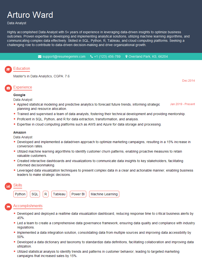
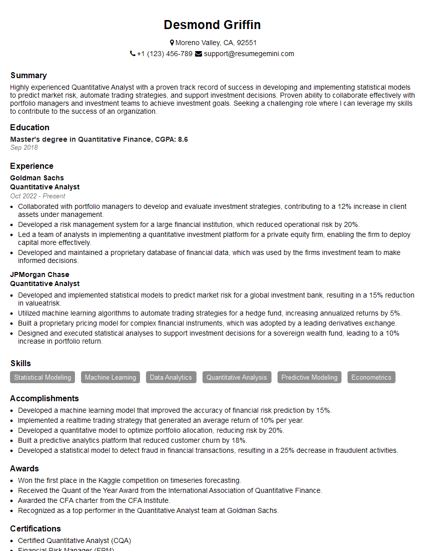
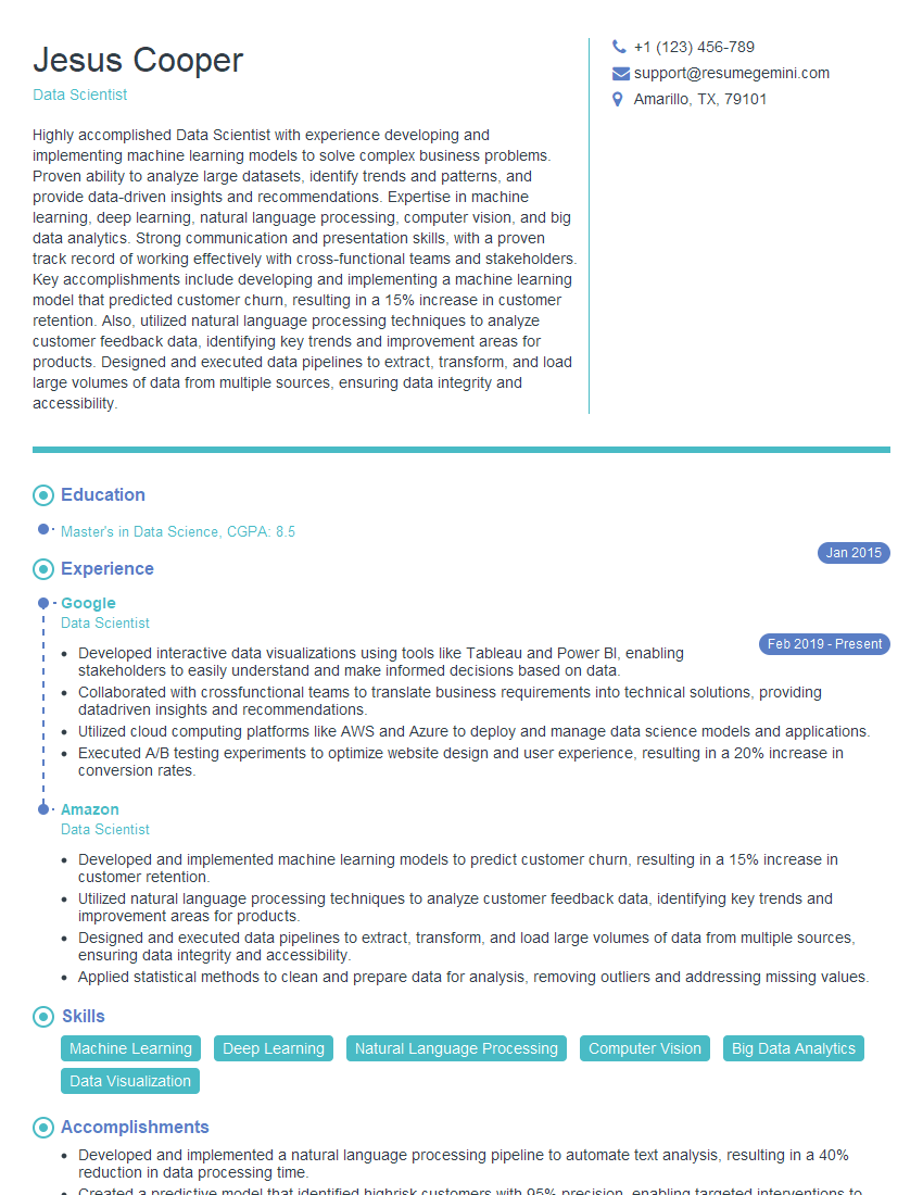
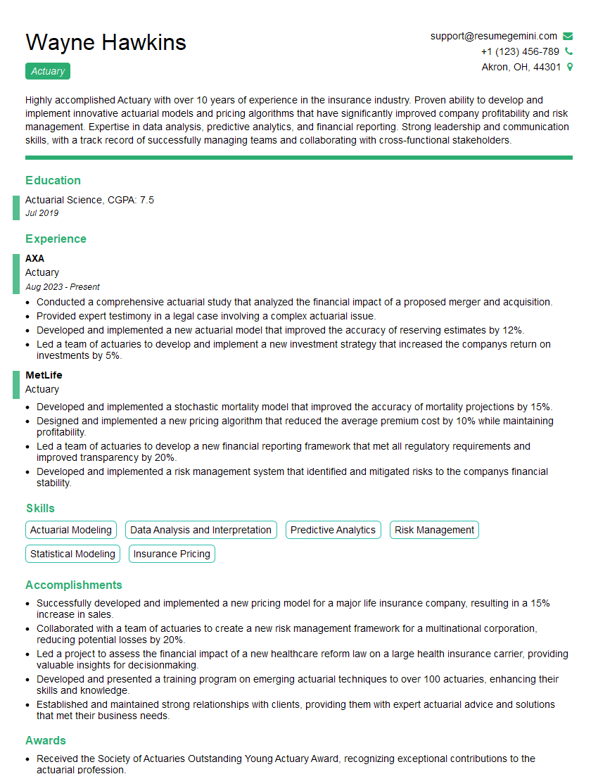
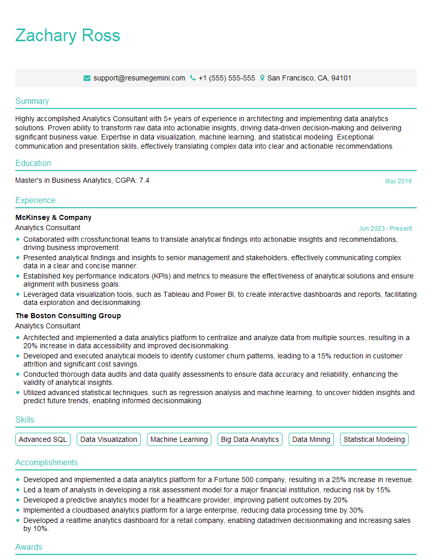
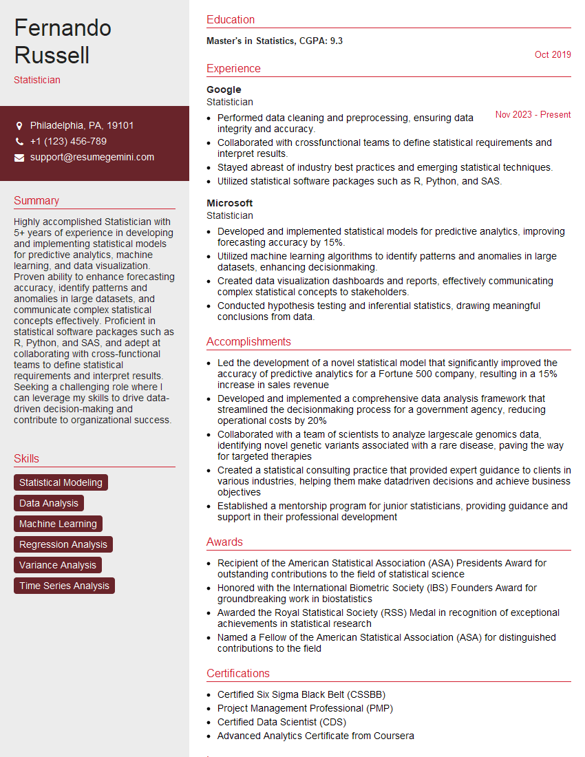
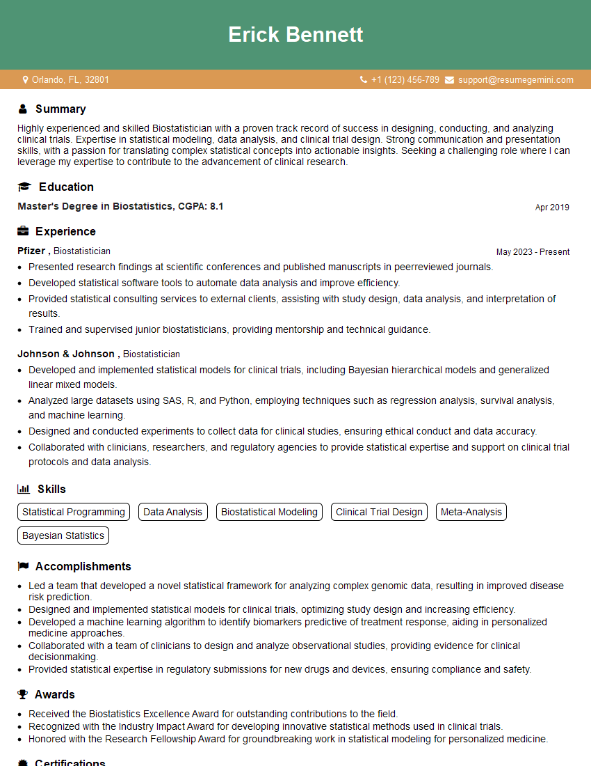
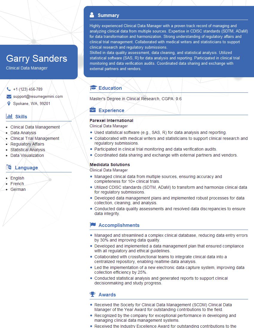
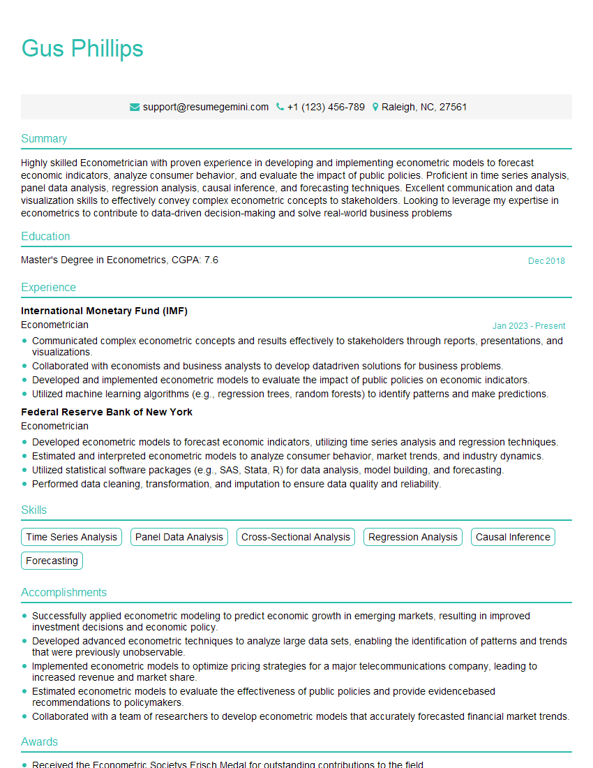
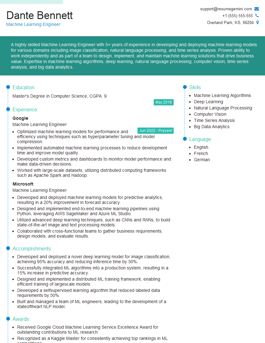
Mastering statistical software like Minitab or R is crucial for career advancement in data analysis, research, and many other fields. It demonstrates a valuable skillset highly sought after by employers. To significantly boost your job prospects, create an ATS-friendly resume that clearly showcases your abilities. ResumeGemini is a trusted resource to help you build a professional and impactful resume that highlights your statistical software expertise. Examples of resumes tailored to Statistical Software (e.g., Minitab, R) roles are available to help guide you.
Explore more articles
Users Rating of Our Blogs
Share Your Experience
We value your feedback! Please rate our content and share your thoughts (optional).
What Readers Say About Our Blog
Hello,
We found issues with your domain’s email setup that may be sending your messages to spam or blocking them completely. InboxShield Mini shows you how to fix it in minutes — no tech skills required.
Scan your domain now for details: https://inboxshield-mini.com/
— Adam @ InboxShield Mini
Reply STOP to unsubscribe
Hi, are you owner of interviewgemini.com? What if I told you I could help you find extra time in your schedule, reconnect with leads you didn’t even realize you missed, and bring in more “I want to work with you” conversations, without increasing your ad spend or hiring a full-time employee?
All with a flexible, budget-friendly service that could easily pay for itself. Sounds good?
Would it be nice to jump on a quick 10-minute call so I can show you exactly how we make this work?
Best,
Hapei
Marketing Director
Hey, I know you’re the owner of interviewgemini.com. I’ll be quick.
Fundraising for your business is tough and time-consuming. We make it easier by guaranteeing two private investor meetings each month, for six months. No demos, no pitch events – just direct introductions to active investors matched to your startup.
If youR17;re raising, this could help you build real momentum. Want me to send more info?
Hi, I represent an SEO company that specialises in getting you AI citations and higher rankings on Google. I’d like to offer you a 100% free SEO audit for your website. Would you be interested?
Hi, I represent an SEO company that specialises in getting you AI citations and higher rankings on Google. I’d like to offer you a 100% free SEO audit for your website. Would you be interested?
good
