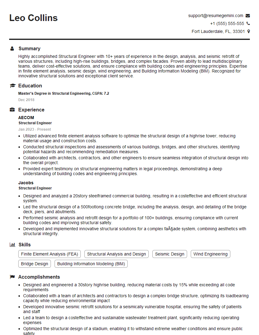
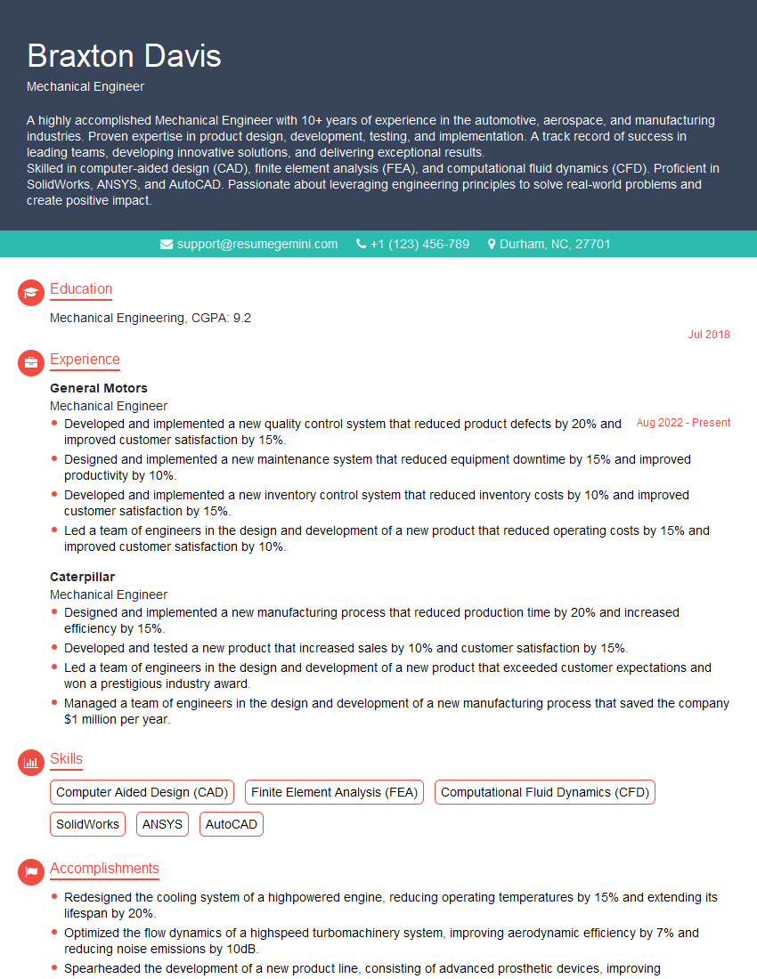
Unlock your full potential by mastering the most common Engineering Math interview questions. This blog offers a deep dive into the critical topics, ensuring you’re not only prepared to answer but to excel. With these insights, you’ll approach your interview with clarity and confidence.
Questions Asked in Engineering Math Interview
Q 1. Explain the concept of eigenvalues and eigenvectors.
Eigenvalues and eigenvectors are fundamental concepts in linear algebra with far-reaching applications in engineering. Imagine a transformation, like stretching or rotating a vector. Eigenvectors are special vectors that, when this transformation is applied, only change in scale (they’re stretched or shrunk), not direction. The factor by which they scale is the eigenvalue.
More formally, for a square matrix A, an eigenvector v satisfies the equation Av = λv, where λ is the eigenvalue (a scalar). Finding eigenvalues and eigenvectors helps us understand the intrinsic properties of a linear transformation, such as its stability or dominant directions.
Example: Consider a rotation matrix. It rotates vectors, but the eigenvectors will be unchanged in direction (except for the trivial zero vector), and the corresponding eigenvalue is always 1. For a stretching transformation along a particular axis, the eigenvectors will lie along that axis and the eigenvalues will indicate the stretching factor along those axes.
In engineering, eigenvalues and eigenvectors are crucial for analyzing vibrations, stability of structures, and principal component analysis in data processing. For instance, in structural analysis, the eigenvalues represent the natural frequencies of a vibrating structure, and the eigenvectors represent the corresponding mode shapes.
Q 2. What are the different methods for solving systems of linear equations?
Solving systems of linear equations is a cornerstone of engineering. Several methods exist, each with its own strengths and weaknesses. The choice depends on factors like the size and structure of the system and computational resources.
- Gaussian Elimination (and Gauss-Jordan): A systematic method for reducing the augmented matrix to row-echelon or reduced row-echelon form. It’s efficient and widely applicable.
- LU Decomposition: This factorizes the coefficient matrix into a lower triangular (L) and an upper triangular (U) matrix. This is particularly useful when solving multiple systems with the same coefficient matrix, as the decomposition needs to be performed only once.
- Matrix Inversion: If the coefficient matrix is invertible, the solution can be directly obtained by multiplying the inverse of the coefficient matrix with the constant vector. Computationally expensive for large systems.
- Cramer’s Rule: Uses determinants to find the solution. Elegant but computationally inefficient for systems with more than a few equations.
- Iterative Methods (Jacobi, Gauss-Seidel, SOR): These methods are particularly suited for large, sparse systems. They provide an approximate solution through successive iterations, converging to the exact solution.
Example: Consider the system: x + 2y = 3 and 3x - y = 1. Gaussian elimination can be used to solve this directly by row operations. LU decomposition would factor the coefficient matrix [[1, 2], [3, -1]] into L and U matrices before back-substitution to find the solution.
Q 3. Describe the process of solving ordinary differential equations (ODEs).
Solving ordinary differential equations (ODEs) involves finding a function that satisfies the given equation. ODEs describe how a quantity changes with respect to a single independent variable (e.g., time or position). The approach depends on the order and type (linear or nonlinear) of the ODE.
- First-Order ODEs: These can often be solved using techniques like separation of variables, integrating factors, or exact equations.
- Higher-Order Linear ODEs with Constant Coefficients: These are solved using characteristic equations, yielding solutions involving exponential and trigonometric functions.
- Nonlinear ODEs: These can be far more challenging. Sometimes, analytical solutions are impossible to find, necessitating numerical methods.
Example: The equation dy/dx = kx is a first-order ODE. Separating variables and integrating gives y = (kx²/2) + C, where C is the constant of integration.
The process often involves finding the general solution (involving arbitrary constants) and then using initial or boundary conditions to determine the particular solution that satisfies the specific problem. Numerical methods such as Euler’s method, Runge-Kutta methods, etc., are employed when analytical solutions are intractable.
Q 4. Explain the Laplace Transform and its applications in solving ODEs.
The Laplace transform is a powerful tool for solving ODEs, particularly those with discontinuous forcing functions or involving initial conditions. It transforms a function of time into a function of a complex variable ‘s’. This transformation simplifies the process of solving ODEs by converting them into algebraic equations, which are easier to solve.
The inverse Laplace transform then converts the solution back into the time domain. The key advantage is its ability to handle initial conditions directly in the transformation process, eliminating the need for separate integration steps.
Example: Consider the ODE dy/dt + y = e^(-t) with initial condition y(0) = 1. Taking the Laplace transform simplifies the problem to an algebraic equation in ‘s’, allowing you to solve for the Laplace transform of y(t). Then the inverse Laplace transform is used to find the solution in the time domain.
Applications include circuit analysis, control systems, and signal processing, where the transform simplifies the analysis of systems responding to time-varying inputs.
Q 5. What are partial differential equations (PDEs) and how are they used in engineering?
Partial differential equations (PDEs) describe functions of multiple independent variables. Unlike ODEs, which involve only one independent variable, PDEs deal with multiple variables, leading to a richer range of solution behavior. For example, a function might vary with both time and spatial coordinates.
Examples of PDEs in engineering:
- Heat equation: Models the distribution of heat (or temperature) in a medium over time.
- Wave equation: Describes the propagation of waves (sound, light, etc.).
- Laplace’s equation: Governs steady-state phenomena like electrostatic fields or fluid flow.
- Navier-Stokes equations: Describe the motion of viscous fluids.
In engineering, PDEs are fundamental for modeling complex systems. For example, designing efficient heat exchangers requires solving the heat equation, while analyzing the vibrations of a bridge involves solving the wave equation.
Q 6. Describe different numerical methods for solving PDEs (e.g., Finite Element Method).
Analytical solutions to PDEs are often difficult or impossible to find, so numerical methods are crucial. These methods approximate the solution by discretizing the domain and applying numerical techniques.
- Finite Difference Method (FDM): Approximates derivatives using difference quotients. Relatively simple to implement but can struggle with complex geometries.
- Finite Element Method (FEM): Divides the domain into smaller elements (triangles, tetrahedra, etc.). More versatile than FDM for handling complex geometries and boundary conditions. It’s widely used in structural analysis, fluid dynamics, and heat transfer.
- Finite Volume Method (FVM): Conserves quantities (like mass or energy) within control volumes. Often used in fluid dynamics and heat transfer simulations.
Finite Element Method (FEM) in detail: The FEM involves dividing the domain into elements, approximating the solution within each element using simple functions (shape functions), and then assembling a system of algebraic equations that represents the entire problem. This system is then solved numerically to obtain the approximate solution at the nodes of the mesh. It is known for its accuracy and ability to handle complex geometries.
Q 7. Explain the concept of Fourier series and its applications.
A Fourier series represents a periodic function as a sum of sine and cosine functions with different frequencies and amplitudes. Imagine taking a complex waveform and breaking it down into its constituent frequencies—this is the essence of a Fourier series.
Any periodic function (within certain constraints) can be approximated by a Fourier series. This is extremely useful in many engineering applications.
Applications:
- Signal processing: Analyzing and processing signals (audio, images, etc.) by decomposing them into their frequency components. This allows for filtering, compression, and other signal manipulations.
- Vibration analysis: Analyzing the vibrational modes of structures by decomposing their vibrations into a superposition of harmonic components.
- Heat transfer: Solving the heat equation in certain cases by expressing the temperature distribution as a Fourier series.
- Partial Differential Equation Solutions: The Fourier series can be a powerful tool for solving some PDEs using the technique of separation of variables.
Example: A square wave can be represented by an infinite sum of sine waves of odd harmonics, with amplitudes decreasing as the frequency increases. This decomposition allows for the analysis and manipulation of the square wave in the frequency domain.
Q 8. How do you use Fourier transforms in signal processing?
Fourier transforms are incredibly useful in signal processing because they allow us to move from the time domain, where we see a signal’s amplitude changing over time, to the frequency domain, where we see the signal’s constituent frequencies and their amplitudes. Think of it like separating a musical chord into its individual notes. In essence, a Fourier transform decomposes a complex signal into a sum of simpler sinusoidal waves.
How it works: A signal, whether it’s an audio recording, a sensor reading, or a financial market trend, can often be represented as a function of time, f(t). The Fourier transform converts this time-domain function into a frequency-domain representation, F(ω), where ω represents the angular frequency. This transformation reveals which frequencies are present in the signal and their relative strengths.
Applications:
- Noise reduction: By identifying and attenuating frequencies associated with noise, we can improve signal clarity.
- Signal compression: Transforming to the frequency domain allows for efficient compression techniques by discarding less significant frequency components (like MP3 compression).
- Image processing: Fourier transforms are fundamental in image analysis, enabling tasks such as edge detection and image filtering.
- Spectral analysis: In fields like engineering, analyzing the frequency content of vibrations in machinery helps in identifying potential problems.
For example, imagine analyzing the vibrations of a jet engine. By performing a Fourier transform on the vibration data, we can pinpoint the frequencies associated with specific engine components. An unusually high amplitude at a particular frequency could indicate a malfunction needing attention.
Q 9. What is the difference between a discrete and continuous Fourier transform?
The core difference lies in whether the input signal is continuous or discrete. A continuous-time Fourier transform (CTFT) operates on continuous functions of time, representing signals that can take on any value at any point in time. The output is also a continuous function of frequency. Think of a smoothly flowing sine wave that extends indefinitely.
On the other hand, a discrete-time Fourier transform (DTFT) handles discrete signals – samples taken at specific intervals. This is how digital signals are represented. While the input is discrete, the output of the DTFT is still continuous in frequency. Imagine the same sine wave but only measured at regular points. The DTFT shows its underlying continuous frequency content.
Now, the discrete Fourier transform (DFT) is very important because it’s computationally feasible. Both the input and output of the DFT are discrete. It is essentially a sampled version of the DTFT. The DFT forms the basis of algorithms like the Fast Fourier Transform (FFT), used extensively in digital signal processing applications because computers work with discrete data.
In summary:
- CTFT: Continuous input, continuous output.
- DTFT: Discrete input, continuous output.
- DFT: Discrete input, discrete output (computationally efficient).
Q 10. Explain the concept of convolution and its applications.
Convolution is a mathematical operation that combines two signals to produce a third signal. Think of it like blending two sounds together. The resulting signal reflects how one signal is modified or ‘smeared’ by the other.
Intuitive Explanation: Imagine you’re throwing a ball at a wall that has some irregularities. The impact of the ball on the wall isn’t just at one point; it spreads out slightly due to the wall’s texture. This spreading is analogous to convolution. The shape of the ball represents one signal (input), the shape of the wall irregularities represents the other (impulse response), and the resulting impact is their convolution.
Mathematical Definition: The convolution of two functions, f(t) and g(t), is typically written as (f * g)(t) and is defined as an integral:
(f * g)(t) = ∫ f(τ)g(t - τ) dτ
This integral represents the overlap between the two functions as one is ‘flipped’ and shifted across the other.
Applications:
- Image blurring: A blurring filter can be represented as a convolution operation, where the input is the original image and the filter is a kernel that ‘smooths’ out the details.
- Signal filtering: Convolution allows for the design of filters that selectively remove or amplify certain frequency components of a signal.
- System response analysis: In control systems, convolution is used to determine the output of a system given its impulse response and input signal.
Q 11. Describe different numerical integration techniques (e.g., Trapezoidal rule, Simpson’s rule).
Numerical integration techniques approximate the definite integral of a function, which represents the area under its curve. This is crucial when analytical integration is difficult or impossible.
Trapezoidal Rule: This method approximates the area under the curve using a series of trapezoids. It’s relatively simple but less accurate than higher-order methods. The area is estimated by summing the areas of trapezoids formed by connecting adjacent points on the function.
∫ab f(x) dx ≈ (b - a)/2 * [f(a) + f(b)] (for a single trapezoid)
For multiple trapezoids, we divide the interval [a, b] into smaller subintervals and apply the formula to each subinterval, summing the results.
Simpson’s Rule: This method uses parabolic approximations instead of straight lines (trapezoids) to fit the curve, yielding a more accurate estimate, particularly for smoother functions. It requires an even number of subintervals.
∫ab f(x) dx ≈ (b - a)/6 * [f(a) + 4f((a+b)/2) + f(b)] (for a single parabolic segment)
Similar to the trapezoidal rule, we divide the interval into smaller subintervals for improved accuracy.
Higher-order methods: More sophisticated methods like Gaussian quadrature offer even greater accuracy by strategically choosing the points at which the function is evaluated.
Error Estimation: The accuracy of these methods depends on the number of subintervals used and the smoothness of the function being integrated. Smaller subintervals generally lead to better accuracy, but increase computational cost. Error analysis techniques are employed to estimate the approximation’s error.
Q 12. How do you solve optimization problems using calculus?
Calculus provides powerful tools for solving optimization problems, which involve finding the maximum or minimum value of a function (objective function) under certain constraints.
Finding Extrema: For unconstrained optimization, we use derivatives. To find local maxima or minima, we set the first derivative of the objective function equal to zero and solve for the critical points. The second derivative test helps classify these critical points as maxima, minima, or saddle points.
Example: Let’s say we want to maximize the area of a rectangle with a fixed perimeter. We can express the area A = xy as a function of x and y. Using the constraint that the perimeter is fixed (2x + 2y = P), we can express y in terms of x and substitute it into the area function. Then, taking the derivative with respect to x, setting it to zero, and solving for x gives the dimensions that maximize the area.
Multivariable Optimization: For functions of multiple variables, we set the partial derivatives with respect to each variable equal to zero to find critical points. Hessian matrices are used to classify the critical points in this case.
Q 13. Explain the method of Lagrange multipliers.
The method of Lagrange multipliers is a powerful technique used to find the extrema of a function subject to constraints. Imagine you’re trying to find the highest point on a hill (your objective function) while staying on a specific path (your constraint).
How it works: Let’s say we want to find the maximum or minimum of a function f(x, y) subject to a constraint g(x, y) = c. The method introduces a new variable, λ (the Lagrange multiplier), and forms the Lagrangian function:
L(x, y, λ) = f(x, y) - λ(g(x, y) - c)
We then find the critical points by taking the partial derivatives of L with respect to x, y, and λ, setting them equal to zero, and solving the resulting system of equations. The solutions provide the candidate points for the extrema.
Geometric Interpretation: At the optimal point, the gradient of the objective function is parallel to the gradient of the constraint function. The Lagrange multiplier λ gives information about how the optimal value of f changes with changes in the constraint c.
Example: Finding the maximum and minimum values of f(x, y) = x2 + y2 subject to the constraint g(x, y) = x + y – 1 = 0. We form the Lagrangian, find the partial derivatives, set them to zero, and solve for x, y, and λ to locate the extrema.
Q 14. What are different types of matrices (e.g., symmetric, skew-symmetric, orthogonal)?
Matrices are fundamental in engineering and possess various properties leading to different classifications:
- Symmetric Matrix: A square matrix where AT = A (the transpose is equal to the original matrix). Elements are symmetric about the main diagonal (aij = aji).
- Skew-Symmetric (or Antisymmetric) Matrix: A square matrix where AT = –A. The elements are antisymmetric about the main diagonal (aij = -aji). The diagonal elements are always zero.
- Orthogonal Matrix: A square matrix where its transpose is equal to its inverse (AT = A-1). This means ATA = I (the identity matrix). Orthogonal matrices represent rotations and reflections in space.
- Diagonal Matrix: A square matrix with non-zero elements only along the main diagonal.
- Identity Matrix: A diagonal matrix with all diagonal elements equal to 1.
- Singular Matrix: A square matrix that doesn’t have an inverse (determinant is zero).
- Invertible Matrix: A square matrix that has an inverse (determinant is non-zero).
These matrix types have significant applications in various areas like linear algebra, computer graphics, and mechanical engineering. For instance, rotation matrices (orthogonal matrices) are crucial for representing rotations in 3D space in computer graphics and robotics.
Q 15. How do you perform matrix operations (e.g., addition, multiplication, inversion)?
Matrix operations are fundamental in linear algebra and are crucial for various engineering applications. Let’s break down addition, multiplication, and inversion.
Matrix Addition: Matrices can be added only if they have the same dimensions (same number of rows and columns). Addition involves adding corresponding elements. For example:
A = [[1, 2], [3, 4]] B = [[5, 6], [7, 8]] A + B = [[6, 8], [10, 12]]Matrix Multiplication: Matrix multiplication is more complex. The number of columns in the first matrix must equal the number of rows in the second matrix. The resulting matrix will have the number of rows from the first matrix and the number of columns from the second. The elements are calculated by taking the dot product of rows and columns. For example:
A = [[1, 2], [3, 4]] B = [[5, 6], [7, 8]] A * B = [[19, 22], [43, 50]]Matrix Inversion: Only square matrices (same number of rows and columns) can be inverted. The inverse of a matrix A, denoted A-1, is a matrix such that A * A-1 = I (the identity matrix, a square matrix with 1s on the diagonal and 0s elsewhere). Finding the inverse involves techniques like Gaussian elimination or using specialized algorithms implemented in software packages like MATLAB or Python’s NumPy. Inversion is used to solve systems of linear equations.
Imagine designing a bridge. The stresses on different parts can be represented by matrices. Matrix operations help determine the overall structural stability by combining and manipulating these stress matrices.
Career Expert Tips:
- Ace those interviews! Prepare effectively by reviewing the Top 50 Most Common Interview Questions on ResumeGemini.
- Navigate your job search with confidence! Explore a wide range of Career Tips on ResumeGemini. Learn about common challenges and recommendations to overcome them.
- Craft the perfect resume! Master the Art of Resume Writing with ResumeGemini’s guide. Showcase your unique qualifications and achievements effectively.
- Don’t miss out on holiday savings! Build your dream resume with ResumeGemini’s ATS optimized templates.
Q 16. What are the applications of linear algebra in engineering problems?
Linear algebra is the backbone of numerous engineering disciplines. Its applications are vast and powerful.
- Structural Engineering: Analyzing stresses and strains in structures (bridges, buildings) using matrix methods to solve systems of linear equations.
- Electrical Engineering: Solving circuit analysis problems, analyzing signal processing algorithms (filtering, transformations), and working with control systems.
- Mechanical Engineering: Analyzing kinematics and dynamics of robots, studying vibrations, and simulating fluid flow using finite element methods (which rely heavily on linear algebra).
- Aerospace Engineering: Simulating flight dynamics, controlling spacecraft maneuvers, and designing aerodynamic surfaces.
- Computer Engineering: Image processing, computer graphics (transformations, projections), and machine learning algorithms.
For instance, in circuit analysis, Kirchhoff’s laws can be expressed as a system of linear equations, readily solved using matrix methods. This provides a concise and efficient approach to determine currents and voltages within complex circuits.
Q 17. Explain the concept of probability and its applications in engineering.
Probability is the branch of mathematics that deals with the likelihood of events occurring. In engineering, it’s essential for modeling uncertainty and risk. Think about designing a self-driving car; probability helps evaluate the chances of different scenarios (e.g., pedestrian detection, collision avoidance) and design robust systems.
Applications in Engineering:
- Reliability Engineering: Predicting the lifespan of components, assessing system failure rates, and optimizing maintenance schedules.
- Quality Control: Determining the probability of defects in manufacturing processes and setting acceptance criteria.
- Signal Processing: Modeling noise and interference in communication systems, designing filters to enhance signal quality.
- Risk Assessment: Evaluating the probability of various hazards and their potential impacts in structural, environmental, and other engineering projects.
For example, in designing a bridge, engineers need to consider the probability of extreme weather events (high winds, floods) and ensure the structure can withstand those conditions with an acceptable level of risk.
Q 18. What are different probability distributions (e.g., normal, exponential, Poisson)?
Several probability distributions model different types of random variables. Here are a few key ones:
- Normal Distribution (Gaussian): A bell-shaped curve, frequently used to model natural phenomena like measurement errors or human heights. It’s characterized by its mean (average) and standard deviation (spread).
- Exponential Distribution: Models the time until an event occurs, often used in reliability engineering to represent the lifespan of a component or the time between failures. It’s characterized by a rate parameter (lambda).
- Poisson Distribution: Models the number of events occurring in a fixed interval of time or space, often used for predicting the number of defects in a manufactured product or the number of customers arriving at a service counter. It’s characterized by a rate parameter (lambda).
- Uniform Distribution: Assigns equal probability to all values within a specific range.
Choosing the right distribution is crucial for accurate modeling. For example, if you are modeling the time to failure of a component, an exponential distribution might be more appropriate than a normal distribution because time to failure can’t be negative.
Q 19. Explain the concept of statistical hypothesis testing.
Statistical hypothesis testing is a formal procedure used to make decisions about a population based on sample data. It involves stating a null hypothesis (H0), which represents the status quo, and an alternative hypothesis (H1), which is what you are trying to prove. You then collect data, perform a statistical test, and determine whether to reject the null hypothesis or fail to reject it.
The process typically includes:
- Formulating Hypotheses: Clearly defining the null and alternative hypotheses.
- Choosing a Significance Level (α): Setting the probability of rejecting the null hypothesis when it’s actually true (Type I error). Common values are 0.05 or 0.01.
- Collecting Data and Performing a Test: Selecting an appropriate statistical test (t-test, chi-squared test, ANOVA, etc.) based on the data type and research question.
- Calculating the p-value: The probability of obtaining the observed results or more extreme results if the null hypothesis is true.
- Making a Decision: If the p-value is less than the significance level (α), you reject the null hypothesis; otherwise, you fail to reject it.
For instance, a manufacturer might test whether a new production process results in fewer defects than the old process. The null hypothesis would be that there’s no difference, and the alternative would be that the new process results in fewer defects.
Q 20. Describe different statistical methods for data analysis.
Numerous statistical methods facilitate data analysis. The choice depends on the nature of the data and the research objectives.
- Descriptive Statistics: Summarizing data using measures like mean, median, mode, standard deviation, and visualization techniques (histograms, box plots).
- Inferential Statistics: Drawing conclusions about a population based on a sample, including hypothesis testing and confidence intervals.
- Regression Analysis: Modeling the relationship between a dependent variable and one or more independent variables (explained in the next answer).
- Analysis of Variance (ANOVA): Comparing the means of three or more groups.
- Time Series Analysis: Analyzing data collected over time to identify trends and patterns.
- Principal Component Analysis (PCA): Reducing the dimensionality of data by identifying the principal components that capture the most variance.
Suppose you’re analyzing customer satisfaction data. Descriptive statistics can summarize average satisfaction scores, while regression analysis could investigate how factors like product quality and customer service relate to overall satisfaction.
Q 21. How do you perform regression analysis?
Regression analysis is a powerful statistical method used to model the relationship between a dependent variable (the outcome you want to predict) and one or more independent variables (predictors).
The goal is to find the best-fitting line (or hyperplane in multiple regression) that describes the relationship. This line is defined by coefficients that represent the effect of each independent variable on the dependent variable. The process typically involves:
- Data Preparation: Cleaning and transforming the data, handling missing values.
- Model Selection: Choosing the appropriate regression model (linear, polynomial, logistic, etc.) based on the data and the nature of the relationship.
- Model Fitting: Estimating the model parameters (coefficients) using techniques like ordinary least squares (OLS).
- Model Evaluation: Assessing the goodness of fit using metrics like R-squared, adjusted R-squared, and residual plots. This helps determine how well the model predicts the dependent variable.
- Prediction: Using the fitted model to predict the dependent variable for new values of the independent variables.
Imagine a civil engineer wants to predict the strength of concrete based on its mix design (cement, water, aggregate proportions). Regression analysis can be used to build a model that relates the mix proportions (independent variables) to the concrete strength (dependent variable).
Q 22. Explain the concept of vector calculus and its applications.
Vector calculus is the branch of mathematics that deals with the differentiation and integration of vector fields. Think of it as extending the familiar concepts of calculus (like derivatives and integrals) to work with quantities that have both magnitude and direction, like forces and velocities. It’s crucial because many physical phenomena, like fluid flow, electromagnetic fields, and heat transfer, are naturally described using vectors.
Applications are widespread: In fluid mechanics, vector calculus helps us understand fluid flow patterns and forces. In electromagnetism, it’s essential for analyzing electric and magnetic fields. In computer graphics, it plays a vital role in modeling surfaces and lighting effects. Even in areas like robotics, vector calculus helps to calculate the movements and trajectories of robots.
Q 23. Describe different types of vector fields (e.g., conservative, solenoidal).
Vector fields are functions that assign a vector to each point in space. Different types exist, with key distinctions:
- Conservative Vector Fields: These fields are path-independent. Imagine walking from point A to point B in a conservative field; the total work done is the same regardless of the path taken. Such fields can be expressed as the gradient of a scalar function (called the potential function). For example, the gravitational field near the Earth’s surface is approximately conservative.
- Solenoidal Vector Fields (or Divergence-free): These fields have zero divergence everywhere. Divergence measures the tendency of a vector field to flow outwards from a point. If the divergence is zero, it means there are no sources or sinks within the field. An example is the magnetic field – magnetic field lines form closed loops, with no beginning or end, implying zero divergence.
- Irrotational Vector Fields (or Curl-free): These fields have zero curl. Curl measures the rotation or circulation of the vector field at a point. Zero curl signifies no rotation. For instance, a uniform electric field is irrotational.
It’s important to note that a field can be both conservative and solenoidal, or neither. The properties of the field dictate the appropriate mathematical tools and techniques for analysis.
Q 24. Explain the concept of line integrals and surface integrals.
Line integrals and surface integrals extend the concept of integration to curves and surfaces, respectively. They’re used to calculate quantities along curves or across surfaces within vector fields.
- Line Integrals: Imagine calculating the work done by a force along a specific path. A line integral sums up the contributions of the vector field along that path. It can be thought of as a generalization of integration along a single variable to integration along a curve. For example, calculating the work done by a force field on a moving particle along a trajectory.
- Surface Integrals: Similar to line integrals but applied to surfaces. Consider calculating the flux of a fluid through a surface. A surface integral sums up the contributions of the vector field across the surface. For example, calculating the total heat flow across the surface of a heat exchanger.
The type of integral (line or surface) and the choice of integrand depend on the specific physical quantity being calculated.
Q 25. How do you apply Green’s theorem, Stokes’ theorem, or the Divergence theorem?
Green’s theorem, Stokes’ theorem, and the Divergence theorem are fundamental theorems of vector calculus that relate integrals over different dimensional domains. They provide powerful tools for simplifying calculations and establishing relationships between different integral forms.
- Green’s Theorem: Relates a line integral around a simple closed curve to a double integral over the plane region bounded by the curve. Useful for simplifying calculations of line integrals in two dimensions.
- Stokes’ Theorem: Relates a line integral around a closed curve to a surface integral over a surface bounded by the curve. Extends Green’s theorem to three dimensions.
- Divergence Theorem: Relates a surface integral over a closed surface to a triple integral over the volume enclosed by the surface. Useful for converting surface integrals into volume integrals, simplifying calculations significantly.
Example (Divergence Theorem): Imagine calculating the total outward flux of a velocity field through a closed surface representing a control volume in fluid mechanics. The Divergence Theorem lets you calculate this flux by integrating the divergence of the velocity field over the volume, often a simpler calculation.
Q 26. Explain complex numbers and their applications in engineering.
Complex numbers extend the real number system by including an imaginary unit, i, defined as i² = -1. They are expressed in the form a + bi, where a and b are real numbers. While seemingly abstract, they are incredibly useful in engineering.
Applications:
- Signal Processing: Complex numbers are fundamental in representing and analyzing signals, particularly sinusoidal signals. The use of Fourier transforms, which rely heavily on complex numbers, allows us to decompose complex signals into simpler components, making signal analysis and processing much easier.
- Control Systems: In the analysis and design of control systems, complex numbers are used to represent transfer functions and analyze system stability and frequency response. The s-plane (complex plane) analysis provides a powerful way to characterize the behavior of control systems.
- Electrical Engineering: Complex numbers are essential for representing impedance, which is the opposition to current flow in electrical circuits. This allows for simpler calculations in AC circuit analysis.
- Fluid Dynamics: Complex analysis can simplify some fluid dynamics problems. The use of complex potential functions offers elegant solutions to problems involving potential flow.
Q 27. Explain the concept of Z-transform and its applications.
The Z-transform is a mathematical tool used to analyze and solve discrete-time signals and systems. It transforms a discrete-time sequence into a complex function of a complex variable, z. Think of it as a discrete-time equivalent of the Laplace transform.
Applications:
- Digital Signal Processing (DSP): The Z-transform is fundamental in DSP for analyzing and designing digital filters, performing spectral analysis, and solving difference equations which arise from the sampled nature of digital systems.
- Control Systems: In discrete-time control systems, the Z-transform is used to analyze the stability and performance of digital control systems by transforming difference equations into algebraic equations.
- Communication Systems: The Z-transform is applied in the analysis of digital communication systems involving discrete signals. For example, to analyze the performance of data transmission over a noisy channel.
Essentially, the Z-transform converts time-domain problems into the frequency domain (using the complex variable ‘z’) for easier analysis and manipulation. This makes it an invaluable tool for many areas of engineering working with discrete data.
Q 28. Describe how you would approach solving a complex engineering problem using mathematical modeling.
Solving complex engineering problems using mathematical modeling involves a structured approach:
- Problem Definition: Clearly define the problem, identifying the key variables, parameters, and assumptions. What are the objectives? What are the constraints?
- Model Development: Based on the problem definition, select appropriate mathematical tools and techniques (e.g., differential equations, finite element analysis, statistical models) to represent the system. This often involves making simplifying assumptions to make the model tractable.
- Model Solution: Solve the mathematical model using analytical or numerical methods. This might involve using software packages for numerical simulations.
- Model Validation and Verification: Compare the model’s predictions to experimental data or known results. Is the model accurate enough? Does it capture the essential behavior of the system?
- Model Refinement: Based on validation results, refine the model to improve its accuracy. This iterative process of refinement continues until satisfactory accuracy is achieved.
- Interpretation and Conclusion: Interpret the model’s results in the context of the original engineering problem. Draw conclusions and make recommendations based on the findings.
Example: Designing a bridge. We might use finite element analysis to model the bridge’s structural behavior under load, using differential equations to model the stress and strain. The solution would provide information on stress levels, deflection, and safety factors, informing the bridge’s design and materials selection. Throughout the process, comparison with experimental data and adjustments would be crucial for validation.
Key Topics to Learn for Your Engineering Math Interview
Acing your engineering math interview requires a solid understanding of both theory and application. Focus your preparation on these key areas:
- Linear Algebra: Mastering vectors, matrices, eigenvalues, and eigenvectors is crucial. Understand their applications in solving systems of equations, representing transformations, and analyzing stability in engineering systems.
- Differential Equations: Develop a strong grasp of solving ordinary and partial differential equations. Practice applying these techniques to model dynamic systems, such as heat transfer, fluid flow, and mechanical vibrations.
- Calculus (Differential and Integral): Ensure a thorough understanding of derivatives, integrals, and their applications in optimization, rate of change problems, and area calculations. Focus on both single and multivariable calculus.
- Probability and Statistics: Develop proficiency in probability distributions, statistical inference, and hypothesis testing. This is particularly relevant for analyzing data, uncertainty, and reliability in engineering projects.
- Numerical Methods: Familiarize yourself with numerical techniques for solving equations and approximating solutions, such as finite difference methods, finite element methods, and iterative solvers. This is vital for handling complex engineering problems that lack analytical solutions.
- Complex Analysis: Understand complex numbers, functions, and their applications in signal processing, control systems, and electromagnetism.
- Transform Methods (Laplace & Fourier): Learn how to use Laplace and Fourier transforms to simplify the analysis of linear systems and signals.
Next Steps: Unlock Your Engineering Career
Mastering engineering math is your key to unlocking exciting career opportunities. It demonstrates a strong analytical foundation and problem-solving ability – highly sought-after skills in the industry. To maximize your chances of landing your dream role, invest time in crafting a compelling, ATS-friendly resume that highlights your skills and experience effectively.
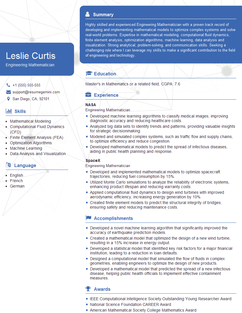
ResumeGemini can help you create a professional and impactful resume tailored to the engineering math field. We provide you with the tools and resources to present yourself in the best possible light, including examples of resumes specifically designed for engineering math professionals. Take the next step towards your successful career journey – build a resume that gets noticed with ResumeGemini.
Explore more articles
Users Rating of Our Blogs
Share Your Experience
We value your feedback! Please rate our content and share your thoughts (optional).
What Readers Say About Our Blog
Very informative content, great job.
good

