Are you ready to stand out in your next interview? Understanding and preparing for Statistical Software (e.g., SPSS, JMP) interview questions is a game-changer. In this blog, we’ve compiled key questions and expert advice to help you showcase your skills with confidence and precision. Let’s get started on your journey to acing the interview.
Questions Asked in Statistical Software (e.g., SPSS, JMP) Interview
Q 1. Explain the difference between descriptive and inferential statistics.
Descriptive statistics summarize the main features of a dataset, giving you a snapshot of your data. Think of it like describing a photo – you’re highlighting key aspects like the overall brightness, central objects, and prominent colors. Inferential statistics, on the other hand, go further. They use sample data to make inferences or predictions about a larger population. It’s like using a small piece of a puzzle to guess what the whole picture looks like.
For example, calculating the average age of participants in a study is descriptive statistics. Using that average age to estimate the average age of the entire population the study participants represent is inferential statistics. Descriptive statistics are about describing what you see in your data, while inferential statistics are about making educated guesses about what you *don’t* see (the broader population).
Q 2. What are the assumptions of a linear regression model?
Linear regression models rely on several key assumptions to ensure accurate and reliable results. These assumptions relate to both the data itself and the relationship between the variables. Violating these assumptions can lead to misleading conclusions.
- Linearity: The relationship between the independent and dependent variables is linear. This means a straight line can reasonably represent the relationship. Scatter plots are crucial for visually assessing this.
- Independence of Errors: The errors (residuals) are independent of each other. This means one data point’s error shouldn’t influence another’s. Autocorrelation can violate this assumption.
- Homoscedasticity: The variance of the errors is constant across all levels of the independent variable. In simpler terms, the spread of the data points around the regression line should be roughly consistent.
- Normality of Errors: The errors are normally distributed. While slight deviations are often tolerable, severe departures can affect the reliability of the results, particularly with smaller sample sizes. Histograms and Q-Q plots are useful for checking this.
- No Multicollinearity: In multiple regression, the independent variables should not be highly correlated with each other. High multicollinearity can inflate standard errors and make it difficult to interpret the individual effects of predictors.
Checking these assumptions is crucial before interpreting the results of a linear regression. SPSS and JMP offer various diagnostic tools to assess these conditions.
Q 3. How do you handle missing data in SPSS/JMP?
Missing data is a common problem in statistical analysis. How you handle it significantly impacts your results. Both SPSS and JMP provide several methods:
- Listwise Deletion (Complete Case Analysis): This simple approach removes any observation with at least one missing value. It’s easy but can lead to substantial data loss and bias if the missing data is not Missing Completely at Random (MCAR).
- Pairwise Deletion: This approach uses all available data for each analysis. For example, if a variable is missing for some participants, it only excludes those participants from analyses involving that variable. It can lead to inconsistencies if different analyses use different subsets of data.
- Imputation: This involves replacing missing values with estimated ones. Methods include mean imputation (replacing with the average), regression imputation (predicting based on other variables), and multiple imputation (creating several plausible imputed datasets). Multiple imputation is generally preferred as it accounts for the uncertainty introduced by imputation.
In SPSS, you can find these options in the ‘Missing Values’ analysis menu. In JMP, you can handle missing data within the modeling platform itself. The best method depends on the nature of your data, the extent of missingness, and the mechanism of missingness (MCAR, MAR, MNAR).
Q 4. Describe different methods for outlier detection.
Outliers are data points that significantly deviate from the rest of the data. Identifying them is important because they can disproportionately influence results and indicate potential errors or interesting subgroups.
- Box Plots: These visually represent data distribution and highlight points falling outside the interquartile range (IQR), often considered outliers (1.5 * IQR above the 3rd quartile or below the 1st quartile).
- Scatter Plots: Useful for identifying outliers in bivariate data, spotting points distant from the main cluster.
- Z-scores: These standardize data, allowing comparison across variables. Points with absolute Z-scores above a threshold (e.g., 3) are often flagged as outliers.
- Cook’s Distance (Regression): In regression analysis, this statistic measures the influence of each data point on the model’s parameters. High Cook’s distance suggests influential outliers.
- Mahalanobis Distance (Multivariate): This measure assesses the distance of a data point from the center of a multivariate data cloud. Large distances indicate potential outliers.
The choice of method depends on the type of data and the context. It’s crucial not to automatically remove outliers without careful investigation. They might represent genuine extreme values or errors that require correction.
Q 5. Explain the concept of p-values and their significance in hypothesis testing.
The p-value is the probability of observing results as extreme as, or more extreme than, the ones obtained, assuming the null hypothesis is true. In simpler terms, it measures the strength of evidence *against* the null hypothesis. The null hypothesis is a statement of no effect or no difference.
A small p-value (typically below a significance level, often 0.05) suggests strong evidence against the null hypothesis. We would then reject the null hypothesis in favor of the alternative hypothesis (which states there *is* an effect or difference). A large p-value suggests insufficient evidence to reject the null hypothesis.
Important Note: A p-value does not indicate the size or importance of an effect. A statistically significant result (low p-value) may still have a small practical effect size. Conversely, a non-significant result (high p-value) doesn’t necessarily mean there’s no effect; it just means the study wasn’t powerful enough to detect it.
Q 6. What are the different types of t-tests and when would you use each?
T-tests compare the means of two groups. There are several types:
- One-sample t-test: Compares the mean of a single group to a known or hypothesized value (e.g., is the average height of students significantly different from 170cm?).
- Independent samples t-test: Compares the means of two independent groups (e.g., is there a significant difference in test scores between males and females?). This assumes the variances of the two groups are equal. If not, a Welch’s t-test is used.
- Paired samples t-test: Compares the means of two related groups (e.g., measuring blood pressure before and after medication). This compares the difference between paired observations.
Choosing the correct t-test depends on the research question and the characteristics of your data. Always check the assumptions of the t-test (e.g., normality of data) before interpreting results.
Q 7. How do you perform ANOVA in SPSS/JMP?
Analysis of Variance (ANOVA) compares the means of three or more groups. Both SPSS and JMP offer straightforward ways to perform ANOVA:
In SPSS: Go to Analyze > Compare Means > One-Way ANOVA. Specify your dependent variable (the outcome you’re measuring) and independent variable (the grouping variable with three or more levels). Post-hoc tests (like Tukey’s HSD) can be selected to determine which specific groups differ if the overall ANOVA is significant.
In JMP: In JMP, you can usually perform ANOVA directly within the Fit Model platform. Select your dependent and independent variables, and JMP will perform the analysis, showing the ANOVA table and relevant statistics. JMP also provides easy access to post-hoc tests.
Regardless of the software, make sure to check the assumptions of ANOVA (normality of data within each group, homogeneity of variances) before drawing conclusions.
Q 8. What are the strengths and weaknesses of using Chi-Square tests?
The Chi-Square test is a powerful statistical tool used to analyze categorical data, determining if there’s a significant association between two categorical variables. Think of it like this: you want to see if ice cream flavor preference (chocolate, vanilla, strawberry) is related to gender (male, female). The Chi-Square test helps you figure that out.
- Strengths: It’s relatively easy to understand and calculate, even without advanced statistical knowledge. It’s widely applicable across various fields, from market research to medical studies. It’s robust to violations of normality assumptions, unlike many parametric tests.
- Weaknesses: It only tells you if there’s an association, not the strength or direction of that association. It can be sensitive to small expected frequencies (cells with low counts), leading to inaccurate results. It doesn’t tell you *why* the association exists; it only identifies that one is present. For example, a Chi-Square test might show an association between ice cream flavor and gender, but doesn’t explain *why* that association exists (e.g., cultural preferences, marketing campaigns).
In SPSS or JMP, you’d typically use the ‘Crosstabs’ procedure, specifying your categorical variables and requesting the Chi-Square statistic.
Q 9. Explain the difference between correlation and causation.
Correlation and causation are often confused, but they are fundamentally different. Correlation simply means that two variables tend to change together. Causation implies that one variable *directly influences* another.
Correlation: Imagine you observe that ice cream sales and crime rates both increase in summer. There’s a correlation – they move together. However, this doesn’t mean that eating ice cream *causes* crime. Both are likely influenced by a third variable: hot weather.
Causation: If you increase the amount of fertilizer used on plants, and observe that plant growth also increases, you might conclude that fertilizer *causes* increased plant growth. This is because you’ve manipulated one variable (fertilizer) and observed a direct effect on the other (growth). Establishing causation requires careful experimental design, often involving controlled experiments and random assignment.
In short, correlation does not equal causation. You can have correlation without causation, but you can’t have causation without correlation.
Q 10. How do you interpret a correlation coefficient?
A correlation coefficient (often denoted as ‘r’) measures the strength and direction of a linear relationship between two variables. It ranges from -1 to +1.
- +1: Perfect positive correlation. As one variable increases, the other increases proportionally.
- 0: No linear correlation. There’s no linear relationship between the variables.
- -1: Perfect negative correlation. As one variable increases, the other decreases proportionally.
The closer the absolute value of ‘r’ is to 1, the stronger the linear relationship. For example, an ‘r’ of 0.8 indicates a strong positive correlation, while an ‘r’ of -0.6 indicates a moderate negative correlation. Remember that correlation doesn’t imply causation; a high correlation merely suggests a linear relationship exists.
In SPSS and JMP, you’d find the correlation coefficient in the output of correlation analysis procedures. You’ll also often see a p-value associated with the correlation, indicating the statistical significance of the relationship.
Q 11. Describe different methods for data visualization in SPSS/JMP.
Both SPSS and JMP offer a wide array of data visualization techniques. Here are a few examples:
- Histograms: Show the distribution of a single continuous variable. Useful for identifying skewness, outliers, and modality.
- Scatter plots: Visualize the relationship between two continuous variables. Useful for identifying correlations and trends.
- Box plots: Compare the distribution of a continuous variable across different groups (categorical variable). Excellent for showing median, quartiles, and outliers.
- Bar charts: Compare the means or frequencies of a categorical variable across different groups.
- Pie charts: Show the proportion of different categories within a whole.
Both SPSS and JMP provide interactive interfaces to create these visualizations, allowing customization of aspects like axis labels, colors, and legends. Specific menu options vary slightly between the two programs, but the fundamental charting capabilities are very similar.
Q 12. How do you create a scatter plot with a regression line in SPSS/JMP?
Creating a scatter plot with a regression line is straightforward in both SPSS and JMP. The specific steps might vary slightly depending on the version, but the general process is consistent:
In SPSS:
- Go to ‘Graphs’ > ‘Legacy Dialogs’ > ‘Scatter/Dot’.
- Select ‘Simple Scatter’.
- Choose your independent (X) and dependent (Y) variables.
- Click ‘OK’.
- To add a regression line, double-click on the scatter plot. In the chart editor, you’ll find options to add a regression line (often under ‘Elements’ or a similar menu).
In JMP:
- Select your independent (X) and dependent (Y) variables.
- Go to ‘Analyze’ > ‘Fit Y by X’.
- JMP will automatically generate a scatter plot. A regression line is typically added by default. You can customize the line and add confidence intervals using the options in the resulting plot.
In both cases, the resulting plot displays the relationship between your two variables, with the regression line providing a visual representation of the best-fitting linear model.
Q 13. How do you perform a logistic regression in SPSS/JMP?
Logistic regression is used when your dependent variable is binary (0 or 1, e.g., success/failure, yes/no). It models the probability of the outcome as a function of one or more predictor variables.
In SPSS:
- Go to ‘Analyze’ > ‘Regression’ > ‘Binary Logistic’.
- Specify your dependent (binary) variable and independent variables.
- Click ‘OK’.
- SPSS will output the regression coefficients, odds ratios, and model fit statistics (e.g., likelihood ratio test, Nagelkerke R-squared).
In JMP:
- Select your dependent (binary) and independent variables.
- Go to ‘Analyze’ > ‘Fit Model’.
- In the ‘Personality’ window, select ‘Logistic’ as the model type.
- JMP will provide similar outputs to SPSS, including parameter estimates and model fit statistics.
The output will help you understand which predictors significantly affect the probability of the outcome and the direction and strength of those effects.
Q 14. Explain the concept of model selection and how it’s performed in SPSS/JMP.
Model selection is the process of choosing the best statistical model from a set of candidate models. The ‘best’ model is typically the one that best balances model fit and parsimony (simplicity). Overly complex models can overfit the data, performing well on the training data but poorly on new data. Simpler models are easier to interpret and generalize better.
In both SPSS and JMP, several methods are used for model selection:
- Stepwise Regression (forward, backward, stepwise): This automated procedure iteratively adds or removes predictors based on their statistical significance.
- Information Criteria (AIC, BIC): These criteria balance model fit and complexity. Models with lower AIC or BIC values are preferred.
- Cross-validation: This technique involves splitting the data into training and testing sets. The model is trained on the training set and evaluated on the testing set, providing an unbiased estimate of its predictive performance.
Both SPSS and JMP provide tools to perform these model selection methods. The specific implementation might differ slightly between the two, but the underlying principles remain the same. The choice of the best model selection method depends on the specific research question and dataset characteristics.
Q 15. How do you assess the goodness of fit of a statistical model?
Assessing the goodness of fit of a statistical model determines how well the model represents the data. We don’t want a model that’s *too* simple (underfitting) and misses important relationships, nor one that’s *too* complex (overfitting) and captures noise instead of signal. The best fit balances simplicity and accuracy.
Several methods exist depending on the model type. For linear regression, we often use:
- R-squared (R²): Represents the proportion of variance in the dependent variable explained by the independent variables. A higher R² suggests a better fit, but it’s not a perfect measure, especially with many predictors.
- Adjusted R-squared: Penalizes the inclusion of unnecessary variables, providing a more reliable measure than R² when comparing models with different numbers of predictors.
- Residual analysis: Examining the residuals (differences between observed and predicted values) can reveal patterns indicating a poor fit. Histograms, Q-Q plots (quantile-quantile plots), and residual plots against fitted values are useful tools. We look for normality, constant variance, and independence of residuals.
- AIC (Akaike Information Criterion) and BIC (Bayesian Information Criterion): These are information criteria that balance model fit with model complexity. Lower AIC and BIC values generally indicate better models.
For other models like logistic regression, we might use metrics like the Hosmer-Lemeshow test, which assesses the goodness of fit by comparing observed and expected frequencies of events across different risk groups. Choosing the appropriate metric depends on the specific model and research question.
Example: In a study predicting customer churn, a high R² in a linear regression model would suggest the model effectively captures factors influencing churn. However, a careful residual analysis is crucial to identify any systematic deviations from the assumptions of the model, which would indicate a poor fit despite a high R².
Career Expert Tips:
- Ace those interviews! Prepare effectively by reviewing the Top 50 Most Common Interview Questions on ResumeGemini.
- Navigate your job search with confidence! Explore a wide range of Career Tips on ResumeGemini. Learn about common challenges and recommendations to overcome them.
- Craft the perfect resume! Master the Art of Resume Writing with ResumeGemini’s guide. Showcase your unique qualifications and achievements effectively.
- Don’t miss out on holiday savings! Build your dream resume with ResumeGemini’s ATS optimized templates.
Q 16. What are different methods for variable selection?
Variable selection aims to identify the most relevant predictors for a model, improving its predictive accuracy and interpretability. Too many variables can lead to overfitting, while too few can result in underfitting. Several methods exist:
- Forward Selection: Starts with no predictors and iteratively adds the predictor that most improves the model fit until adding more variables doesn’t significantly improve the fit.
- Backward Elimination: Starts with all predictors and iteratively removes the least significant predictor until removing variables significantly worsens the fit.
- Stepwise Selection: A combination of forward and backward selection, iteratively adding and removing variables based on their significance.
- Best Subset Selection: Considers all possible combinations of predictors and selects the best-fitting subset based on a chosen criterion (e.g., adjusted R²).
- Regularization methods (LASSO, Ridge): Shrink the coefficients of less important predictors towards zero, effectively performing variable selection while reducing overfitting. These are particularly useful with high-dimensional data.
The choice of method depends on factors such as the number of predictors, the size of the dataset, and the computational resources available. Best subset selection is computationally intensive for a large number of variables.
Example: In a marketing campaign effectiveness model, stepwise selection might identify email open rate, click-through rate, and website engagement as the key predictors of conversion, while excluding less impactful variables like time spent on social media.
Q 17. Explain the concept of multicollinearity and how to address it.
Multicollinearity occurs when two or more predictor variables in a regression model are highly correlated. This makes it difficult to isolate the individual effects of each predictor on the outcome variable, leading to unstable and unreliable coefficient estimates. Imagine trying to determine the individual impact of flour and sugar on the taste of a cake when you always add them in a fixed ratio – you can’t disentangle their independent effects.
Consequences of multicollinearity include inflated standard errors of the regression coefficients (making it harder to find statistically significant results), unstable coefficient estimates that may flip sign with minor changes in the data, and difficulty interpreting the meaning of the coefficients.
Addressing multicollinearity involves:
- Assessing multicollinearity: Use variance inflation factors (VIFs) – a VIF > 5 or 10 is often considered an indication of problematic multicollinearity. Also look at the correlation matrix of predictors.
- Removing redundant variables: If two variables are highly correlated, remove one of them. Choose the variable with a less clear theoretical relationship with the outcome or the one that leads to a better model fit.
- Combining correlated variables: Create a composite variable by averaging or summing the correlated predictors.
- Principal Component Analysis (PCA): Transform the correlated variables into a set of uncorrelated principal components. This is useful for dimensionality reduction when dealing with a large number of highly correlated predictors.
- Regularization techniques: Ridge regression and LASSO regression can mitigate the impact of multicollinearity by shrinking the coefficients.
Example: In a model predicting house prices, if both square footage and number of bedrooms are highly correlated, removing one or creating a composite variable (e.g., ‘size’ = square footage/number of bedrooms) can resolve multicollinearity.
Q 18. How do you handle categorical variables in regression analysis?
Categorical variables, representing groups or categories rather than numerical values, need special handling in regression analysis. They can’t be directly included as is. The most common approach is to use dummy coding (also known as one-hot encoding):
Dummy coding: For a categorical variable with k levels, create k-1 dummy variables. Each dummy variable represents a level of the categorical variable, and takes a value of 1 if the observation belongs to that level and 0 otherwise. One level is omitted (the reference category) to avoid perfect multicollinearity. The omitted category’s effect is implicitly captured in the intercept.
Example: If we have a categorical variable ‘color’ with levels ‘red,’ ‘green,’ and ‘blue,’ we create two dummy variables: ‘red’ (1 if red, 0 otherwise) and ‘green’ (1 if green, 0 otherwise). ‘Blue’ is the reference category. The regression coefficient for ‘red’ indicates the difference in the outcome variable between red and blue, while the coefficient for ‘green’ represents the difference between green and blue.
Software like SPSS and JMP automatically handle dummy coding when you include categorical predictors in regression analysis. The choice of the reference category can influence interpretation; the best choice depends on the research question.
Q 19. What are the different types of sampling methods?
Sampling methods determine how we select a subset of individuals from a population for study. The choice of sampling method impacts the generalizability of the findings. Key types include:
- Simple Random Sampling: Each member of the population has an equal chance of being selected. This is straightforward but may not be representative if the population is heterogeneous.
- Stratified Random Sampling: The population is divided into strata (subgroups) based on relevant characteristics (e.g., age, gender). A random sample is then drawn from each stratum, ensuring representation from all subgroups.
- Cluster Sampling: The population is divided into clusters (e.g., geographical areas, schools). A random sample of clusters is selected, and all members within the selected clusters are included in the study.
- Systematic Sampling: Every kth member of the population is selected after a random starting point. Simple but can be problematic if there’s a pattern in the population that aligns with the sampling interval.
- Convenience Sampling: Selecting participants based on their easy availability. This is prone to bias and should be avoided whenever possible.
Example: To study student satisfaction, stratified random sampling might be used to ensure representation from different academic years and majors, whereas cluster sampling could involve selecting a few schools and surveying all students within those schools.
Q 20. Explain the central limit theorem.
The Central Limit Theorem (CLT) is a fundamental concept in statistics. It states that the distribution of the sample means of a large number of independent, identically distributed random variables, regardless of the shape of the original population distribution, will approximate a normal distribution. The approximation improves as the sample size increases.
This is incredibly useful because it allows us to make inferences about a population even if we don’t know its true distribution. We can use the normal distribution’s properties to construct confidence intervals and conduct hypothesis tests.
Conditions for CLT: The CLT holds under some conditions, primarily independence and a sufficiently large sample size (typically n ≥ 30). The size requirement is less strict if the population distribution is already close to normal.
Example: Suppose we want to estimate the average height of all adults in a city. We collect a large random sample of heights. Even if the population height distribution is not perfectly normal (it might be slightly skewed), the distribution of sample means will be approximately normal, according to the CLT. We can then use this to estimate the population mean height and its confidence interval.
Q 21. Describe your experience with data cleaning and preparation.
Data cleaning and preparation are crucial steps before any analysis. My experience includes handling missing values, outliers, and inconsistencies, transforming variables, and ensuring data integrity.
Missing data: I use various techniques depending on the nature and extent of missing data, such as deletion (listwise or pairwise), imputation using mean, median, or mode for numerical variables, more sophisticated methods like k-nearest neighbors (k-NN) or multiple imputation for more complex patterns. The best strategy depends on the data and the extent of missingness. I always carefully document the method used.
Outliers: I identify outliers using box plots, scatter plots, or z-scores. I investigate the causes of outliers – are they errors or genuine extreme values? If errors, they are corrected or removed; if genuine, I might consider transformations (e.g., log transformation) or robust statistical methods that are less sensitive to outliers.
Data transformation: I use transformations (log, square root, etc.) to meet the assumptions of statistical models (e.g., normality, linearity) or to improve model fit.
Data consistency: I ensure consistency in data coding, units, and formats across the dataset. This frequently involves using scripting languages like R or Python for efficient processing and manipulation of large datasets. I always create detailed documentation explaining my cleaning and preparation steps for reproducibility and transparency.
Example: In a medical study, I would carefully handle missing values in patient records, deciding whether to impute missing dosages based on patient history or remove patients with extensive missing data. I would also flag and investigate any unusually high or low blood pressure readings, determining whether they were errors or indicated a unique medical condition.
Q 22. How familiar are you with different data manipulation techniques?
Data manipulation is the cornerstone of any successful statistical analysis. It involves a wide range of techniques aimed at cleaning, transforming, and preparing data for analysis. My familiarity spans several key areas:
- Data Cleaning: This includes handling missing values (using imputation methods like mean substitution, regression imputation, or more sophisticated techniques depending on the data), identifying and removing outliers, and correcting inconsistencies in data entry.
- Data Transformation: This often involves converting data into a more suitable format for analysis. Examples include standardizing variables (z-scores), creating dummy variables for categorical data, and log transforming skewed data to achieve normality.
- Data Reduction: Techniques like principal component analysis (PCA) and factor analysis can reduce the dimensionality of large datasets, making analysis more manageable and efficient. This is crucial when dealing with high-dimensional data where the ‘curse of dimensionality’ can significantly impact model performance.
- Data Aggregation: Combining data from multiple sources or summarizing data into meaningful aggregates (e.g., calculating means, medians, and sums for different groups) is another essential aspect.
For instance, in a recent project analyzing customer purchase behavior, I had to deal with missing values for income. Instead of simply removing these entries (which would lead to a significant loss of data), I employed multiple imputation using chained equations, creating several plausible income values based on other variables and then analyzing the results across these imputations to gauge the robustness of my conclusions.
Q 23. Explain your experience with creating and interpreting reports from statistical analyses.
Creating and interpreting statistical reports is a crucial skill, going beyond simply generating numbers. It involves communicating findings clearly and concisely to both technical and non-technical audiences. My experience encompasses:
- Report Structure: I always structure reports logically, starting with a clear introduction outlining the objectives and methodology, followed by the results (presented with tables, charts, and graphs), and concluding with a discussion of the implications and limitations.
- Visualization: I leverage various visualization techniques (histograms, scatter plots, box plots, etc.) in SPSS and JMP to effectively communicate complex data patterns. I choose the most appropriate visualization based on the type of data and the message I want to convey.
- Interpretation: I go beyond simply presenting statistics; I interpret the results in the context of the research question, highlighting significant findings and explaining any unexpected results. I always consider the potential biases and limitations of the analysis.
- Software Proficiency: I’m proficient in using SPSS and JMP to generate publication-ready tables and charts directly from the analysis, minimizing the need for manual data transfer and reducing the risk of errors.
For example, in a recent client project involving market research, I used JMP to create interactive dashboards that allowed clients to explore the data dynamically. This enabled them to understand the nuances of the findings more effectively than a static report could have.
Q 24. How proficient are you in using SPSS syntax or JMP scripting?
I possess strong proficiency in both SPSS syntax and JMP scripting. While I can effectively use the graphical user interfaces (GUIs) of both software packages, I recognize the power and efficiency of scripting for complex analyses and repetitive tasks.
- SPSS Syntax: I can write efficient SPSS syntax for data manipulation, statistical modeling (regression, ANOVA, etc.), and report generation. This allows for reproducibility and automation of analyses.
- JMP Scripting (JSL): I’m comfortable using JSL to automate tasks, create custom functions, and develop interactive visualizations within JMP. This enables me to tailor the analysis workflow to specific project needs.
/* Example SPSS Syntax for calculating a new variable */ COMPUTE newvar = var1 + var2. EXECUTE.
/* Example JSL for creating a custom function */ Function MyFunction(x){ return x^2; };
I frequently use scripting to streamline repetitive analyses, such as processing large datasets or performing simulations, which significantly enhances efficiency and reduces potential human error.
Q 25. Describe a time you had to troubleshoot a statistical analysis.
During a project analyzing survey data, I encountered unexpected negative correlations between variables that were theoretically expected to be positively correlated. This raised concerns about the validity of the data or the analysis.
My troubleshooting process involved:
- Data Inspection: I meticulously examined the data for errors, inconsistencies, or outliers that might have skewed the results. I used histograms and scatter plots to visualize the data distribution and identify potential issues.
- Re-examination of the Methodology: I reviewed the survey design and question wording to ensure there were no ambiguities or biases that might have influenced the responses.
- Alternative Analyses: I explored alternative analytical techniques to see if the unexpected findings persisted. For instance, I used robust regression methods that are less sensitive to outliers.
- Consultation: I consulted with colleagues experienced in survey methodology to discuss potential explanations for the unexpected findings and to gain alternative perspectives.
Ultimately, through this systematic troubleshooting process, we identified a flaw in the survey design that led to the unexpected negative correlation. The revised survey and subsequent analysis produced results consistent with the expected theoretical relationships.
Q 26. How do you ensure the accuracy and reliability of your statistical analysis?
Ensuring accuracy and reliability in statistical analysis is paramount. My approach is multifaceted and includes:
- Data Validation: I thoroughly check the data for accuracy and consistency, using both automated checks and manual inspection. This includes verifying data entry, identifying and addressing missing values, and flagging potential outliers.
- Appropriate Statistical Methods: I carefully select statistical methods appropriate for the type of data and the research question, ensuring the assumptions of each method are met. This might involve transformations or alternative analytical techniques.
- Sensitivity Analysis: When appropriate, I conduct sensitivity analyses to assess the impact of model assumptions and potential biases on the results. This helps to understand how robust the findings are to changes in the underlying data or assumptions.
- Peer Review: I actively seek feedback from colleagues on my analyses to identify potential errors or biases. A fresh pair of eyes can often identify issues that I might have overlooked.
- Documentation: I maintain detailed documentation of my analysis process, including the data cleaning steps, the statistical methods used, and the interpretation of the results. This makes the analysis reproducible and transparent.
By adhering to these principles, I strive to produce reliable and trustworthy results that can inform decision-making with confidence.
Q 27. Explain your experience working with large datasets.
I have extensive experience working with large datasets, leveraging both the capabilities of SPSS and JMP, and employing efficient data handling strategies. This includes:
- Data Management Techniques: I utilize techniques like data sampling, data partitioning, and efficient data structures to manage large datasets effectively. Sampling allows for faster analysis without compromising results in many instances.
- High-Performance Computing: For exceptionally large datasets that exceed the capacity of standard desktop computing, I’m familiar with using distributed computing techniques or cloud-based solutions (like AWS or Azure) to perform the analysis efficiently.
- Data Warehousing and Databases: I have experience working with relational databases (like SQL Server or MySQL) to query and extract data for analysis. This allows seamless integration with large, structured datasets.
- Data Mining Techniques: I’m also familiar with data mining techniques to extract meaningful insights from complex, large datasets. This often involves predictive modeling using techniques like decision trees, logistic regression, or support vector machines.
For example, in a project involving millions of customer transactions, I employed a combination of sampling and parallel processing techniques within SPSS to perform an analysis of customer segmentation, identifying specific segments which respond positively to targeted marketing campaigns, enabling the company to maximize its ROI. This optimized both speed and efficiency.
Q 28. What are some of the ethical considerations in data analysis?
Ethical considerations are paramount in data analysis. My commitment to ethical practices includes:
- Data Privacy and Confidentiality: I always adhere to strict data privacy protocols, ensuring the confidentiality of sensitive data. This involves anonymizing data when possible and following all relevant regulations (e.g., GDPR, HIPAA).
- Data Integrity and Accuracy: I prioritize maintaining the integrity and accuracy of the data, ensuring data is handled responsibly and without bias. This involves rigorous data validation and cleaning procedures.
- Avoiding Bias: I’m aware of the potential for bias in both data collection and analysis, actively working to mitigate these biases. This involves carefully considering the sample selection process and applying appropriate statistical methods.
- Transparency and Reproducibility: I maintain transparent and reproducible analyses, clearly documenting my methods and making the data and code available when appropriate. This ensures accountability and allows others to scrutinize the findings.
- Appropriate Interpretation: I avoid misrepresenting the findings or drawing unwarranted conclusions from the analysis. The interpretation of results must be grounded in the data and the methodology employed.
Ethical data handling is not just a matter of compliance; it’s a fundamental aspect of responsible scientific practice. I understand that the misuse of data can have significant consequences, and I always strive to act with integrity and uphold the highest ethical standards.
Key Topics to Learn for Statistical Software (e.g., SPSS, JMP) Interview
- Data Import and Cleaning: Mastering techniques for importing data from various sources (CSV, Excel, databases), handling missing values, and identifying/correcting outliers. Practical application: Preparing real-world datasets for analysis.
- Descriptive Statistics: Calculating and interpreting measures of central tendency (mean, median, mode), variability (standard deviation, variance), and distribution. Practical application: Summarizing key features of a dataset to inform further analysis.
- Inferential Statistics: Understanding and applying hypothesis testing (t-tests, ANOVA, Chi-square), regression analysis (linear, logistic), and confidence intervals. Practical application: Drawing conclusions about a population based on sample data.
- Data Visualization: Creating effective charts and graphs (histograms, box plots, scatter plots) to communicate data insights clearly. Practical application: Presenting findings in a compelling and understandable manner.
- Model Building and Evaluation: Developing and evaluating statistical models, understanding model assumptions, and interpreting model outputs. Practical application: Building predictive models or identifying significant relationships between variables.
- Specific Software Features (SPSS/JMP): Familiarizing yourself with the unique functionalities and strengths of the chosen software. This includes understanding the software’s interface, syntax, and specific procedures relevant to your target role. Practical application: Efficiently performing analyses within the chosen software environment.
- Data Interpretation and Reporting: Clearly communicating statistical findings and their implications in a concise and professional manner. Practical application: Preparing reports and presentations for stakeholders.
Next Steps
Mastering statistical software like SPSS and JMP is crucial for career advancement in data analysis, research, and many other fields. Proficiency in these tools demonstrates valuable skills to potential employers and significantly increases your job prospects. To maximize your chances, focus on building a strong, ATS-friendly resume that highlights your abilities. ResumeGemini is a trusted resource to help you craft a professional and impactful resume that showcases your skills effectively. Examples of resumes tailored to Statistical Software (e.g., SPSS, JMP) expertise are available to guide you.

Business Analyst Resume Sample

Market Research Analyst Resume Sample

Data Analyst Resume Sample

Quantitative Analyst Resume Sample

Data Scientist Resume Sample

Research Scientist Resume Sample

Actuary Resume Sample

Analytics Consultant Resume Sample

Operations Research Analyst Resume Sample
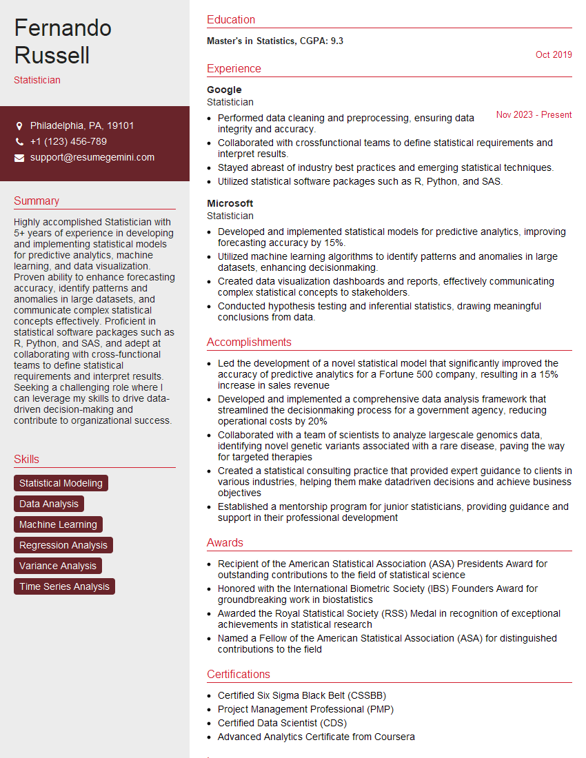
Statistician Resume Sample

Biostatistician Resume Sample

Clinical Data Analyst Resume Sample
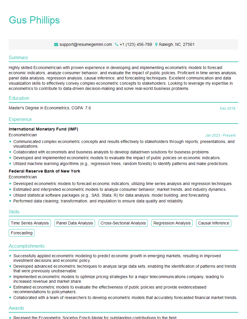
Econometrician Resume Sample

Survey Researcher Resume Sample

Machine Learning Engineer Resume Sample
Explore more articles
Users Rating of Our Blogs
Share Your Experience
We value your feedback! Please rate our content and share your thoughts (optional).
What Readers Say About Our Blog
Very informative content, great job.
good