The thought of an interview can be nerve-wracking, but the right preparation can make all the difference. Explore this comprehensive guide to Mathematics and Science Proficiency interview questions and gain the confidence you need to showcase your abilities and secure the role.
Questions Asked in Mathematics and Science Proficiency Interview
Q 1. Explain the concept of statistical significance.
Statistical significance assesses whether an observed effect in data is likely due to a real effect rather than random chance. Imagine flipping a coin 10 times and getting 7 heads. Is this unusual? Not really. But if you flipped it 1000 times and got 700 heads, that’s highly suspicious – it suggests the coin might be biased. Statistical significance helps us quantify this suspicion.
It’s usually expressed using a p-value. A small p-value (typically less than 0.05) suggests that the observed result is unlikely to have occurred by random chance alone, indicating statistical significance. The threshold (0.05) is arbitrary and can be adjusted based on the context, but it provides a standard benchmark.
For example, in a clinical trial testing a new drug, a statistically significant result would mean that the observed difference in outcomes between the treatment group and the control group is unlikely due to random variation and suggests the drug has a real effect.
Q 2. Describe different types of hypothesis testing.
Hypothesis testing involves formulating a hypothesis (a statement about a population parameter) and then using sample data to assess the plausibility of that hypothesis. There are several types:
- One-sample t-test: Compares the mean of a single sample to a known population mean. Example: Testing if the average height of students in a school is different from the national average.
- Two-sample t-test: Compares the means of two independent samples. Example: Comparing the effectiveness of two different teaching methods by comparing the average test scores of two groups of students.
- Paired t-test: Compares the means of two related samples (e.g., before and after measurements on the same individuals). Example: Measuring blood pressure before and after administering a medication to the same patients.
- ANOVA (Analysis of Variance): Compares the means of three or more groups. Example: Comparing the yield of crops using different fertilizers.
- Chi-square test: Used to analyze categorical data and determine if there’s a significant association between two categorical variables. Example: Determining if there’s a relationship between smoking and lung cancer.
The choice of test depends on the type of data and the research question.
Q 3. What is the difference between correlation and causation?
Correlation measures the strength and direction of a relationship between two variables, while causation implies that one variable directly influences the other. Correlation does not imply causation.
Example: Ice cream sales and crime rates might be positively correlated (both increase in summer). This doesn’t mean eating ice cream causes crime, or vice versa. A third variable, temperature, is likely the cause of both increases.
To establish causation, you need to demonstrate a cause-and-effect relationship, often through controlled experiments or strong observational studies with careful consideration of confounding variables. Correlation is simply an indication that two variables change together; it doesn’t explain why.
Q 4. How would you interpret a p-value?
The p-value is the probability of observing the obtained results (or more extreme results) if the null hypothesis is true. The null hypothesis is a statement of no effect or no difference. A small p-value suggests that the observed results are unlikely to have occurred by chance alone, providing evidence against the null hypothesis.
For example, a p-value of 0.03 means there’s a 3% chance of observing the data if there was truly no effect. This is often considered strong evidence against the null hypothesis (leading to rejection of the null hypothesis), although the interpretation should be made in context with the research question and the consequences of a wrong decision.
It’s crucial to remember that a non-significant p-value (e.g., >0.05) does not prove the null hypothesis is true; it simply means there’s insufficient evidence to reject it.
Q 5. Explain the central limit theorem.
The Central Limit Theorem (CLT) states that the distribution of the sample means of a sufficiently large number of independent, identically distributed random variables will be approximately normal, regardless of the shape of the original distribution.
Imagine repeatedly taking samples from any population (even if it’s skewed or non-normal). As the sample size increases, the distribution of the sample means will approach a normal distribution. This is incredibly useful because many statistical methods rely on the assumption of normality.
Example: If you measure the heights of individuals in a population that isn’t normally distributed, the average height from many large samples will follow a normal distribution. This allows us to use normal distribution-based tests (like t-tests) even when the original data isn’t normally distributed, provided the sample size is large enough.
Q 6. What are the assumptions of linear regression?
Linear regression models the relationship between a dependent variable and one or more independent variables using a linear equation. Several assumptions underpin its validity:
- Linearity: There’s a linear relationship between the dependent and independent variables.
- Independence: Observations are independent of each other.
- Homoscedasticity: The variance of the errors is constant across all levels of the independent variable(s).
- Normality: The errors are normally distributed.
- No multicollinearity: Independent variables are not highly correlated with each other (in multiple regression).
Violations of these assumptions can lead to biased or inefficient estimates and inaccurate inferences. Diagnostic plots and tests are used to assess the validity of these assumptions.
Q 7. Describe different methods for handling missing data.
Missing data is a common problem in statistical analysis. Several methods exist for handling it:
- Listwise deletion: Removing any observation with missing values. This is simple but can lead to substantial loss of information if many observations have missing data and may introduce bias if the missingness is not random.
- Pairwise deletion: Using available data for each analysis. This avoids losing as much data as listwise deletion but can lead to inconsistencies.
- Imputation: Replacing missing values with estimated values. Methods include mean imputation (replacing with the mean of the observed values), regression imputation (predicting missing values based on other variables), and multiple imputation (creating several plausible imputed datasets).
- Maximum likelihood estimation (MLE): A statistical method that estimates model parameters by maximizing the likelihood function, which incorporates the missing data mechanism.
The best approach depends on the pattern and nature of the missing data, the size of the dataset, and the research question. It’s crucial to understand the mechanisms of missing data (Missing Completely at Random (MCAR), Missing at Random (MAR), Missing Not at Random (MNAR)) to choose the most appropriate method.
Q 8. Explain the concept of Bayesian inference.
Bayesian inference is a powerful statistical method that allows us to update our beliefs about the probability of an event based on new evidence. Instead of simply calculating probabilities from observed data alone (like frequentist statistics), Bayesian inference starts with a prior belief – our initial estimate of the probability. This prior is then combined with new data (likelihood) using Bayes’ Theorem to produce a posterior belief – a refined estimate reflecting both our prior knowledge and the observed data. Imagine you’re trying to determine if a coin is fair. Your prior might be that it’s equally likely to be fair (50/50 heads/tails) or biased. After flipping the coin 10 times and observing 8 heads, the likelihood of observing this data given a fair coin is low. Applying Bayes’ theorem, your posterior belief will shift towards the coin being biased. This iterative process of updating beliefs allows for a more nuanced understanding of probability in the face of uncertainty.
Bayes’ Theorem is formally expressed as: P(A|B) = [P(B|A) * P(A)] / P(B), where P(A|B) is the posterior probability of A given B, P(B|A) is the likelihood of B given A, P(A) is the prior probability of A, and P(B) is the prior probability of B (often calculated using the law of total probability).
Bayesian inference finds wide application in fields like medical diagnosis (updating the probability of a disease given symptoms), spam filtering (updating the probability of an email being spam based on its content), and machine learning (e.g., in Naive Bayes classifiers).
Q 9. What is the difference between supervised and unsupervised machine learning?
The key difference between supervised and unsupervised machine learning lies in the nature of the data used for training. In supervised learning, the data is labeled; that is, each data point is associated with a known outcome or target variable. The algorithm learns to map inputs to outputs based on these labeled examples. Think of teaching a child to identify different fruits – you show them apples, oranges, and bananas (inputs) and tell them the name of each fruit (output/label). The algorithm learns to predict the fruit name given an image of the fruit.
Unsupervised learning, on the other hand, uses unlabeled data. The algorithm’s task is to discover patterns, structures, or relationships in the data without any predefined labels. An example is customer segmentation – grouping customers based on purchasing behavior without pre-defined customer segments. The algorithm might discover clusters of customers with similar purchasing patterns, revealing valuable insights.
In essence, supervised learning aims to predict, while unsupervised learning aims to explore and understand.
Q 10. Describe different types of machine learning algorithms.
Machine learning algorithms span a vast landscape, categorized by their learning style (supervised, unsupervised, reinforcement) and specific approach. Some key types include:
- Supervised Learning:
- Linear Regression: Predicts a continuous target variable using a linear relationship.
- Logistic Regression: Predicts a binary or categorical target variable.
- Support Vector Machines (SVMs): Finds an optimal hyperplane to separate data points into different classes.
- Decision Trees: Builds a tree-like model to classify or regress data.
- Random Forests: An ensemble method that combines multiple decision trees.
- Naive Bayes: A probabilistic classifier based on Bayes’ theorem.
- Unsupervised Learning:
- K-Means Clustering: Partitions data into k clusters based on similarity.
- Hierarchical Clustering: Builds a hierarchy of clusters.
- Principal Component Analysis (PCA): Reduces the dimensionality of data while retaining important information.
- Reinforcement Learning:
- Q-learning: An algorithm that learns optimal actions in an environment through trial and error.
This is not an exhaustive list, but it highlights some of the most commonly used algorithms, each with strengths and weaknesses depending on the problem at hand.
Q 11. Explain the concept of overfitting and underfitting.
Overfitting and underfitting are two common problems encountered in machine learning, both stemming from the model’s ability to generalize to unseen data. Overfitting occurs when a model learns the training data too well, including noise and outliers. It performs exceptionally well on the training data but poorly on new, unseen data. Imagine a student memorizing the answers to a practice exam rather than understanding the underlying concepts; they’ll do well on the practice exam but poorly on the actual exam.
Underfitting, conversely, occurs when a model is too simple to capture the underlying patterns in the data. It performs poorly on both training and test data. This is like a student only skimming the textbook; they’ll do poorly on both the practice and the actual exam.
Techniques to address overfitting include regularization (adding penalties to complex models), cross-validation (evaluating model performance on multiple subsets of the data), and using simpler models. Underfitting can be addressed by using more complex models, adding more features, or improving the model’s training process.
Q 12. How do you evaluate the performance of a machine learning model?
Evaluating the performance of a machine learning model is crucial to ensure its reliability and effectiveness. The choice of evaluation metrics depends on the type of problem (classification, regression, clustering) and the specific goals. Common techniques include:
- Holdout method: Splitting the data into training and testing sets.
- Cross-validation: Evaluating the model on multiple subsets of the data to get a more robust estimate of performance. k-fold cross-validation is a popular technique.
- Confusion matrix: A table showing the counts of true positive, true negative, false positive, and false negative predictions for classification problems.
- Metrics: Accuracy, precision, recall, F1-score, AUC-ROC (Area Under the Receiver Operating Characteristic curve) for classification problems; Mean Squared Error (MSE), Root Mean Squared Error (RMSE), R-squared for regression problems.
The choice of metric should always be aligned with the specific business needs. For example, in medical diagnosis, minimizing false negatives (missing a disease) might be more important than maximizing overall accuracy.
Q 13. Explain the difference between accuracy, precision, and recall.
Accuracy, precision, and recall are crucial metrics for evaluating the performance of classification models, particularly when dealing with imbalanced datasets (where one class has significantly more instances than another). Let’s illustrate with the example of a spam detection model.
- Accuracy: The overall correctness of the model; the percentage of correctly classified emails (spam or not spam) out of the total number of emails. A high accuracy might be misleading in the case of skewed data.
- Precision: Out of all the emails the model classified as spam, what proportion were actually spam? High precision means a low rate of false positives (non-spam emails mistakenly classified as spam).
- Recall: Out of all the emails that were actually spam, what proportion did the model correctly identify as spam? High recall means a low rate of false negatives (spam emails mistakenly classified as not spam).
The best choice of metric depends on the context. If misclassifying spam as not spam has serious consequences (e.g., missing critical information), recall is more important. If misclassifying non-spam as spam is more problematic (e.g., annoying users with false alerts), precision is more important.
Q 14. What is the difference between a Type I and Type II error?
Type I and Type II errors are both related to hypothesis testing. They represent different types of mistakes we can make when deciding whether to reject or fail to reject a null hypothesis. Consider a medical test for a disease:
- Type I error (False Positive): Rejecting the null hypothesis when it is actually true. In our example, this would mean concluding that a patient has the disease when they actually do not. The probability of making a Type I error is denoted by α (alpha).
- Type II error (False Negative): Failing to reject the null hypothesis when it is actually false. In our example, this means concluding that a patient does not have the disease when they actually do. The probability of making a Type II error is denoted by β (beta).
The consequences of Type I and Type II errors can vary greatly depending on the context. In some situations, a Type I error might be more costly (e.g., unnecessary medical treatment), while in others, a Type II error might be far more serious (e.g., delayed treatment for a serious disease). The choice of significance level (α) balances the risk of these two types of errors.
Q 15. Describe the process of hypothesis testing.
Hypothesis testing is a crucial statistical method used to make inferences about a population based on sample data. It involves formulating a hypothesis (a statement about the population), collecting data, and then determining whether the data provides enough evidence to reject the hypothesis in favor of an alternative. Think of it like a trial – you start by assuming innocence (the null hypothesis), and the evidence (data) needs to be strong enough to convince you of guilt (rejecting the null hypothesis).
The process typically involves these steps:
- Formulate a null hypothesis (H0) and an alternative hypothesis (H1 or Ha): The null hypothesis is a statement of no effect or no difference, while the alternative hypothesis is what you’re trying to prove. For example, if testing a new drug, H0 might be ‘the drug has no effect on blood pressure,’ and H1 might be ‘the drug lowers blood pressure’.
- Choose a significance level (α): This represents the probability of rejecting the null hypothesis when it’s actually true (Type I error). Commonly, α is set at 0.05, meaning there’s a 5% chance of making a Type I error.
- Collect data and calculate a test statistic: This statistic measures how far your sample data deviates from what you’d expect under the null hypothesis. Examples include t-tests, z-tests, and chi-squared tests, chosen based on the type of data and the research question.
- Determine the p-value: The p-value is the probability of obtaining results as extreme as, or more extreme than, the observed data, assuming the null hypothesis is true. A low p-value (typically less than α) suggests strong evidence against the null hypothesis.
- Make a decision: If the p-value is less than α, you reject the null hypothesis; otherwise, you fail to reject the null hypothesis. Remember, failing to reject doesn’t prove the null hypothesis is true, it just means there’s not enough evidence to reject it.
Example: A researcher wants to test if a new fertilizer increases crop yield. The null hypothesis is that the fertilizer has no effect, and the alternative is that it increases yield. After collecting data, a t-test is performed, resulting in a p-value of 0.02. Since 0.02 < 0.05, the researcher rejects the null hypothesis and concludes that the fertilizer likely increases crop yield.
Career Expert Tips:
- Ace those interviews! Prepare effectively by reviewing the Top 50 Most Common Interview Questions on ResumeGemini.
- Navigate your job search with confidence! Explore a wide range of Career Tips on ResumeGemini. Learn about common challenges and recommendations to overcome them.
- Craft the perfect resume! Master the Art of Resume Writing with ResumeGemini’s guide. Showcase your unique qualifications and achievements effectively.
- Don’t miss out on holiday savings! Build your dream resume with ResumeGemini’s ATS optimized templates.
Q 16. Explain the concept of probability distributions.
A probability distribution describes the likelihood of obtaining different possible values for a random variable. It essentially maps each possible value of the variable to its probability of occurrence. Imagine rolling a six-sided die – the probability distribution would show that each number (1 to 6) has a probability of 1/6.
There are two main types:
- Discrete Probability Distributions: These describe discrete variables, which can only take on specific, separate values (e.g., the number of heads when flipping a coin, the number of cars passing a point on a road in an hour). Examples include the binomial distribution (probability of getting a certain number of successes in a fixed number of trials) and the Poisson distribution (probability of a given number of events occurring in a fixed interval of time or space).
- Continuous Probability Distributions: These describe continuous variables, which can take on any value within a given range (e.g., height, weight, temperature). Examples include the normal distribution (bell curve), the exponential distribution (time until an event occurs), and the uniform distribution (all values within a range are equally likely).
Importance: Probability distributions are fundamental in statistics and many scientific fields. They allow us to model randomness, make predictions, and test hypotheses. For instance, knowing the probability distribution of rainfall helps in designing irrigation systems, and understanding the distribution of customer arrival times helps optimize staffing in a service industry.
Q 17. What is the difference between a discrete and continuous variable?
The key difference lies in the values they can take:
- Discrete Variable: A discrete variable can only take on a finite number of values or a countably infinite number of values. These values are often whole numbers and usually represent counts or categories. Examples include the number of students in a class (15, 20, 25…), the number of cars in a parking lot, or the number of defective items in a batch.
- Continuous Variable: A continuous variable can take on any value within a given range. It’s often measured rather than counted and usually involves some degree of precision. Examples include height (1.75 meters, 1.82 meters…), weight (70.5 kg, 72.2 kg…), temperature (25.3°C, 26.1°C…), or time.
Analogy: Think of counting whole apples versus measuring the weight of apples. The number of apples is a discrete variable, while the weight is a continuous variable. You can have 3 apples or 4 apples, but you can’t have 3.5 apples. However, an apple can weigh 0.25 kg, 0.251 kg, 0.2512 kg, etc. The possibilities are infinite within the range of possible apple weights.
Q 18. Explain the concept of differential equations.
A differential equation is an equation that relates a function to its derivatives. In simpler terms, it describes how a quantity changes over time or with respect to another variable. It often involves the rate of change of one variable with respect to another. For instance, it could describe the rate at which a population grows, the speed of a falling object, or the spread of a disease.
The order of a differential equation is determined by the highest derivative present. A first-order differential equation involves only the first derivative, while a second-order differential equation involves the second derivative, and so on. Differential equations can be ordinary (involving only one independent variable) or partial (involving multiple independent variables).
Example: The equation dy/dx = 2x is a first-order ordinary differential equation. It states that the rate of change of y with respect to x is equal to 2x. Solving this equation would give us the function y(x).
Q 19. Describe different methods for solving differential equations.
Several methods exist for solving differential equations, the choice depending on the type and complexity of the equation. Here are a few common techniques:
- Separation of Variables: This method is applicable to first-order equations where the variables can be separated on different sides of the equation. It involves integrating both sides to find the solution.
- Integrating Factors: This method is used for first-order linear differential equations. An integrating factor is multiplied to the equation to make it integrable.
- Substitution: Sometimes, a substitution of variables can simplify a differential equation, making it solvable by other methods.
- Homogeneous Equations: Homogeneous equations have a specific form that allows for a particular substitution to simplify the solution process.
- Linear Differential Equations with Constant Coefficients: These equations have characteristic equations whose roots can be used to find the general solution.
- Numerical Methods: For complex differential equations that lack analytical solutions, numerical methods like Euler’s method or Runge-Kutta methods can provide approximate solutions.
Example (Separation of Variables): Consider the equation dy/dx = xy. We can separate variables to get (1/y)dy = xdx. Integrating both sides yields ln|y| = (1/2)x² + C, where C is the constant of integration. Solving for y gives y = Ae(x²/2), where A = ±eC.
Q 20. Explain the concept of integration.
Integration is the reverse process of differentiation. While differentiation finds the rate of change of a function, integration finds the function whose derivative is given. It’s essentially finding the area under a curve.
There are two main types:
- Definite Integral: This calculates the area under a curve between two specified limits. It yields a numerical value. For example, the definite integral
∫ab f(x) dxrepresents the area under the curve f(x) from x = a to x = b. - Indefinite Integral: This finds the family of functions whose derivative is the given function. It yields a function plus a constant of integration. For example, the indefinite integral
∫ f(x) dxrepresents the set of functions whose derivative is f(x).
Fundamental Theorem of Calculus: This theorem connects differentiation and integration, showing that differentiation and integration are inverse operations.
Applications: Integration is used to calculate areas, volumes, work, and many other quantities in physics, engineering, and other fields. For instance, it’s used to calculate the total distance traveled from a velocity function or the total work done by a force.
Q 21. What are the applications of calculus in your field?
Calculus is indispensable in my field, finding application in various ways:
- Modeling Dynamic Systems: Differential equations, a core concept in calculus, are used to model systems that change over time, such as population growth, chemical reactions, and the spread of diseases. Understanding these dynamics requires both differentiation (to find rates of change) and integration (to find accumulated effects).
- Optimization Problems: Calculus provides tools for finding maximum and minimum values of functions. This is crucial in optimizing resource allocation, maximizing profits, or minimizing costs in various settings.
- Data Analysis and Statistics: Calculus plays a vital role in probability theory and statistical inference. Concepts like probability density functions and cumulative distribution functions are defined using integrals. Many statistical tests and estimation techniques rely on calculus.
- Numerical Methods: Approximation techniques, often based on calculus, are essential when dealing with complex equations or systems that don’t have analytical solutions.
- Signal Processing: Calculus underpins signal processing techniques, such as Fourier transforms, which are used to analyze and manipulate signals in fields like image processing and communication systems.
Example: In a biological model of population growth, the rate of change of population (dP/dt) might be modeled as a function of the current population size (P) and available resources. Solving the resulting differential equation using calculus allows us to predict future population sizes.
Q 22. Describe different methods for solving systems of linear equations.
Solving systems of linear equations involves finding the values of variables that satisfy all equations simultaneously. Several methods exist, each with its strengths and weaknesses. Let’s explore a few:
Substitution Method: Solve one equation for one variable and substitute this expression into the other equation(s). This reduces the number of variables until you can solve for one, then back-substitute to find the others. For example, consider the system:
x + y = 5x - y = 1We can solve the first equation for x:
x = 5 - y. Substituting this into the second equation gives(5 - y) - y = 1, which simplifies to2y = 4, soy = 2. Substituting this back intox = 5 - ygivesx = 3. The solution is (3, 2).Elimination Method (or Linear Combination): Multiply equations by constants to make the coefficients of one variable opposites. Adding the equations then eliminates that variable, allowing you to solve for the remaining variable. For the same system above, we can add the two equations directly:
(x + y) + (x - y) = 5 + 1, simplifying to2x = 6, sox = 3. Then substitute back into either original equation to findy = 2.Matrix Methods (Gaussian Elimination, Gauss-Jordan Elimination): These methods use matrices to represent the system of equations. Gaussian elimination transforms the augmented matrix into row echelon form, while Gauss-Jordan elimination goes further to reduced row echelon form, directly yielding the solution. These are particularly efficient for larger systems.
Cramer’s Rule: This method uses determinants to solve for each variable. While elegant, it becomes computationally expensive for large systems.
The choice of method depends on the specific system and personal preference. For small systems, substitution or elimination are often quickest. For larger systems, matrix methods are generally more efficient and less prone to error.
Q 23. Explain the concept of vectors and matrices.
Vectors and matrices are fundamental concepts in linear algebra. Think of a vector as a directed line segment—it has both magnitude (length) and direction. We can represent vectors using ordered lists of numbers called components. For instance, v = [2, 3] represents a vector in two dimensions. Matrices are rectangular arrays of numbers arranged in rows and columns. They can be thought of as collections of vectors.
Vectors: Applications include representing physical quantities like forces and velocities, or representing data points in higher dimensions. Vector operations include addition, subtraction, scalar multiplication, and dot product (which measures the alignment of two vectors). For example, adding two vectors v = [1, 2] and w = [3, 4] results in v + w = [4, 6].
Matrices: Matrices are used extensively in linear transformations (like rotations, scaling, and shearing), solving systems of linear equations (as mentioned before), and representing data in various forms. Matrix operations include addition, subtraction, multiplication, and finding inverses. Matrix multiplication isn’t commutative (AB ≠ BA in general), which is an important distinction.
Imagine a spreadsheet; each row could represent a product, and each column could represent a characteristic (price, quantity, etc.). This structured data naturally maps onto a matrix representation.
Q 24. What are the applications of linear algebra in your field?
Linear algebra is indispensable in numerous fields, including my own work in [mention your field, e.g., data science, engineering, physics]. Some key applications include:
Data analysis and machine learning: Matrices and vectors are used to represent data sets and perform operations like dimensionality reduction (Principal Component Analysis), classification (linear classifiers), and regression analysis. Eigenvalues and eigenvectors are fundamental concepts in these applications.
Computer graphics and image processing: Linear transformations (represented by matrices) are used to rotate, scale, and shear images. Image compression techniques often rely on linear algebra.
Network analysis: Matrices can represent connections between nodes in a network (e.g., social networks, transportation networks), allowing analysis of centrality measures, community detection, etc.
Quantum mechanics: Linear algebra is the mathematical language of quantum mechanics. Quantum states are represented as vectors, and quantum operators as matrices.
Numerical analysis and simulations: Solving systems of differential equations often involves linear algebra techniques.
Essentially, whenever you have structured data or relationships that can be represented linearly, linear algebra provides powerful tools for analysis and manipulation.
Q 25. Describe the principles of thermodynamics.
Thermodynamics is the study of energy and its transformations. It’s governed by four fundamental laws:
Zeroth Law: If two systems are each in thermal equilibrium with a third system, then they are in thermal equilibrium with each other. This establishes the concept of temperature.
First Law (Conservation of Energy): Energy cannot be created or destroyed, only transferred or changed from one form to another. The change in internal energy of a system is equal to the heat added to the system minus the work done by the system: ΔU = Q – W.
Second Law: The total entropy of an isolated system can only increase over time, or remain constant in ideal cases where the system is in a steady state or undergoing a reversible process. This implies that natural processes tend towards disorder (increased entropy).
Third Law: The entropy of a perfect crystal at absolute zero temperature is zero. This provides a reference point for entropy measurements.
These laws have profound implications for understanding energy efficiency, predicting the spontaneity of reactions, and designing various technologies. For example, understanding the second law is crucial in designing efficient power plants and engines.
Q 26. Explain the concept of chemical equilibrium.
Chemical equilibrium describes a state in a reversible chemical reaction where the rates of the forward and reverse reactions are equal. This means the concentrations of reactants and products remain constant over time, although the reaction is still ongoing. It’s a dynamic equilibrium, not a static one.
The equilibrium constant (Keq) is a value that quantifies the relative amounts of reactants and products at equilibrium. A large Keq indicates that the equilibrium favors products, while a small Keq indicates that the equilibrium favors reactants. Factors affecting equilibrium include temperature, pressure (for gaseous reactions), and concentration.
Le Chatelier’s principle states that if a change of condition is applied to a system in equilibrium, the system will shift in a direction that relieves the stress. For example, increasing the concentration of a reactant will shift the equilibrium towards products.
Understanding chemical equilibrium is essential in many industrial processes, such as designing chemical reactors and optimizing reaction conditions for maximum product yield.
Q 27. Describe different types of chemical reactions.
Chemical reactions can be classified in several ways, based on the changes involved:
Combination (Synthesis): Two or more reactants combine to form a single product. Example:
2H₂ + O₂ → 2H₂ODecomposition: A single reactant breaks down into two or more products. Example:
2H₂O₂ → 2H₂O + O₂Single Displacement (Substitution): One element replaces another in a compound. Example:
Zn + 2HCl → ZnCl₂ + H₂Double Displacement (Metathesis): Two compounds exchange ions to form two new compounds. Example:
AgNO₃ + NaCl → AgCl + NaNO₃Acid-Base Reactions: An acid reacts with a base to form a salt and water (neutralization). Example:
HCl + NaOH → NaCl + H₂ORedox (Oxidation-Reduction) Reactions: Involve the transfer of electrons between reactants. One reactant is oxidized (loses electrons), and the other is reduced (gains electrons). Example:
Fe + Cu²⁺ → Fe²⁺ + Cu
These categories aren’t mutually exclusive; some reactions can fall into multiple categories.
Q 28. Explain the concept of genetic algorithms.
Genetic algorithms are a type of optimization algorithm inspired by the process of natural selection. They’re used to find approximate solutions to complex problems that are difficult or impossible to solve using traditional methods.
The algorithm starts with a population of candidate solutions (individuals), each represented as a string of parameters (chromosomes). These solutions are then evaluated using a fitness function, which measures how well each solution solves the problem. The algorithm then selects the fittest individuals to reproduce, creating new solutions through genetic operators like:
Crossover: Combining parts of the chromosomes from two parent solutions to create offspring.
Mutation: Randomly changing parts of a chromosome to introduce diversity.
This process of selection, crossover, and mutation is repeated over many generations, gradually improving the fitness of the population and converging towards an optimal or near-optimal solution. Genetic algorithms are particularly useful for problems with large search spaces, non-linearity, or multiple local optima.
A classic example is finding the optimal shape of an airplane wing to minimize drag. The parameters (wingspan, curvature, etc.) would be encoded in the chromosome, and the drag would be the fitness function. The algorithm would iterate, creating and evaluating wing designs until it converges on a near-optimal design.
Key Topics to Learn for Mathematics and Science Proficiency Interview
- Mathematical Modeling: Understanding how to translate real-world problems into mathematical equations and interpret the results. Practical applications include data analysis, forecasting, and simulation.
- Statistical Analysis: Proficiency in descriptive and inferential statistics, including hypothesis testing and regression analysis. Essential for data-driven decision making in various scientific fields.
- Scientific Method & Experimental Design: A strong grasp of the scientific method, including hypothesis formulation, experimental design, data collection, analysis, and interpretation. Crucial for research and development roles.
- Calculus & Differential Equations: Understanding fundamental calculus concepts and their applications in physics, engineering, and other scientific disciplines. Practice solving various types of differential equations.
- Linear Algebra & Matrix Operations: Familiarity with vectors, matrices, and linear transformations. This is vital for computer science, data science, and many engineering fields.
- Physics Fundamentals: A solid understanding of classical mechanics, thermodynamics, electromagnetism, and potentially quantum mechanics, depending on the specific role. Relate theoretical concepts to real-world phenomena.
- Chemistry Fundamentals: Knowledge of basic chemical principles, including stoichiometry, chemical bonding, and reaction kinetics. Consider exploring organic chemistry or biochemistry depending on the specific job requirements.
- Problem-Solving Techniques: Develop your ability to approach complex problems systematically, breaking them down into smaller, manageable parts. Practice different problem-solving strategies and algorithms.
Next Steps
Mastering Mathematics and Science Proficiency is crucial for career advancement in numerous high-demand fields. A strong foundation in these areas opens doors to exciting opportunities in research, development, technology, and data science. To maximize your job prospects, create an ATS-friendly resume that highlights your skills and achievements effectively. ResumeGemini is a trusted resource to help you build a professional and impactful resume that showcases your expertise. Examples of resumes tailored to Mathematics and Science Proficiency are available on ResumeGemini to guide you in creating your own compelling application materials.

Environmental Scientist Resume Sample

Quantitative Analyst Resume Sample

Data Scientist Resume Sample

Research Scientist Resume Sample

Geologist Resume Sample

Actuary Resume Sample

Cryptographer Resume Sample

Mathematician Resume Sample

Operations Research Analyst Resume Sample

Statistician Resume Sample

Bioinformatician Resume Sample

Biostatistician Resume Sample

Aerospace Engineer Resume Sample

Chemical Engineer Resume Sample
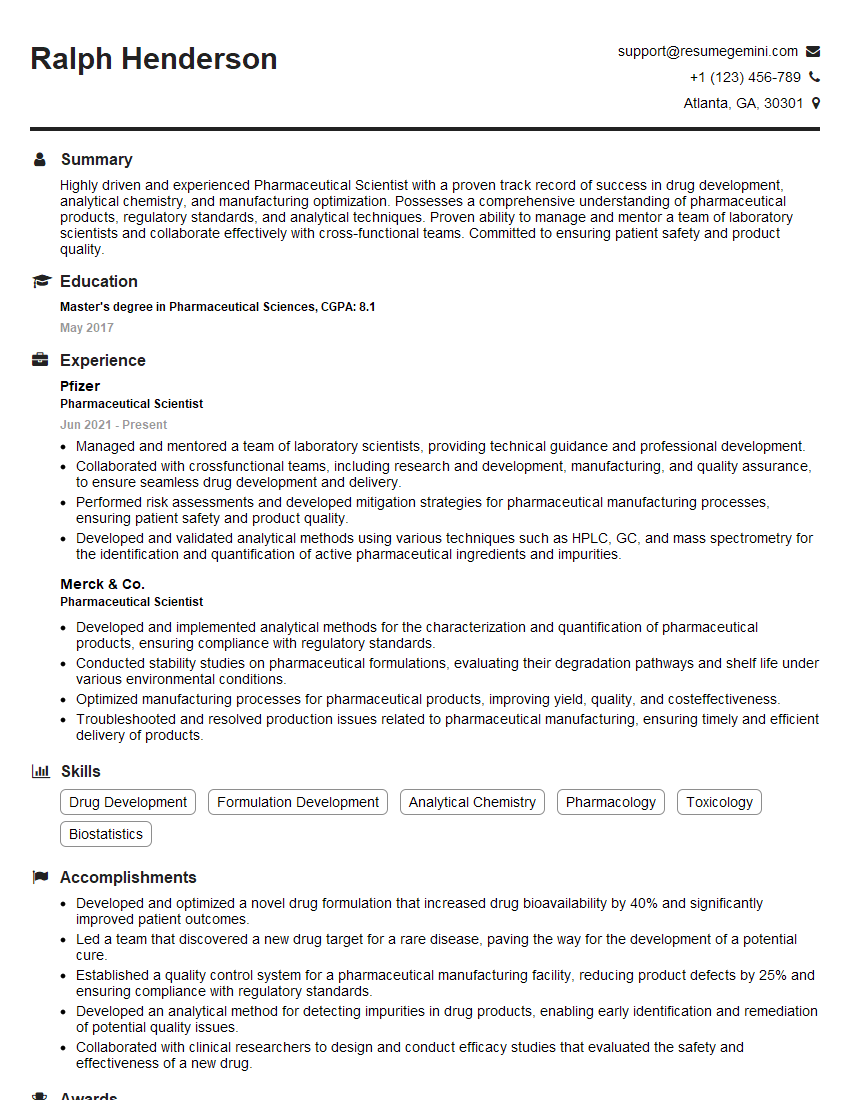
Pharmaceutical Scientist Resume Sample

Chemist Resume Sample

Computational Biologist Resume Sample

Medical Scientist Resume Sample
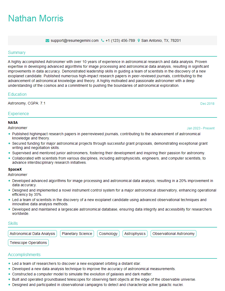
Astronomer Resume Sample

Nuclear Scientist Resume Sample

Physicist Resume Sample

Materials Scientist Resume Sample
- Environmental Scientist
- Quantitative Analyst
- Data Scientist
- Research Scientist
- Geologist
- Actuary
- Cryptographer
- Mathematician
- Operations Research Analyst
- Statistician
- Bioinformatician
- Biostatistician
- Aerospace Engineer
- Chemical Engineer
- Pharmaceutical Scientist
- Chemist
- Computational Biologist
- Medical Scientist
- Astronomer
- Nuclear Scientist
- Physicist
- Materials Scientist
Explore more articles
Users Rating of Our Blogs
Share Your Experience
We value your feedback! Please rate our content and share your thoughts (optional).
What Readers Say About Our Blog
Very informative content, great job.
good